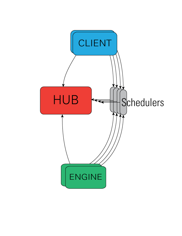
from IPython import parallel in 15 min
Based on the Parallel Monto-Carlo options pricing from IPython.parallel examples.
This notebook shows how to use IPython.parallel to do Monte-Carlo options pricing in parallel.
We will compute the price of a large number of options for different strike prices and volatilities.
Few words about IPython ecosystem
from IPython.display import HTML
HTML('<iframe src=http://ipython.org/index.html width=1024 height=350></iframe>')
HTML('<iframe src=http://nbviewer.ipython.org/ width=1024 height=350></iframe>')
HTML('<iframe src=http://continuum.io/downloads width=1024 height=350></iframe>')
Have we got a cluster running?
First we my need to create a profile (default will be there by default)
ipython profile create --parallel --profile=yourProfileName
You can start it by using the IPython Notebook's Clusters tab
Or by calling (of it form):
ipcluster start -n 4
Or the combination of
ipcontroller --ip=192.169.X.Y and ipengine
Where you want really want your controller to start up first, whilst engines will checks the ipcontroller-engine.json file it generates (you will copy it from say .ipython/profile_default/security/ipcontroller-engine.json to location from where engine will read it).
If you are on restricted network, don't worry there is support for SSH tunneling
from IPython.parallel import Client
c = Client()
c.history, c.ids
([], [0, 1, 2, 3, 4, 5, 6, 7])
dv = c[:]
print(type(dv))

lv = c.load_balanced_view()
print(type(lv))

dv.results.items()
<class 'IPython.parallel.client.view.DirectView'>
<class 'IPython.parallel.client.view.LoadBalancedView'>
[]
Passing data around
ar = dv.scatter('x', range(64),block=True)
print(type(ar))

ar = dv.scatter('x', range(1024*1024*30),block=False)
ar.get(), ar.progress, ar.elapsed, ar.ready(), ar.serial_time, ar.wall_time
<type 'NoneType'>
([None, None, None, None, None, None, None, None],
 8,
 1.509833,
 True,
 1.4056050000000002,
 1.509833)
l = c[4]['x']
print(4, min(l), max(l), len(l))
l = c[6]['x']
print(6, min(l), max(l), len(l))

c[0].push(dict(x=[0]))
l= dv.pull('x',targets=0,block=True)
print(0, min(l), max(l), len(l))

l = c[7].pull('x').get()
print(7, min(l), max(l), len(l))

dv.push(dict(x=[1]))
dv.gather('x').get()
(4, 15728640, 19660799, 3932160)
(6, 23592960, 27525119, 3932160)
(0, 0, 0, 1)
(7, 27525120, 31457279, 3932160)
[1, 1, 1, 1, 1, 1, 1, 1]
import gc
gc.collect()
0
with c[:].sync_imports():
    import gc

%px gc.collect()
importing gc on engine(s)
Out[0:1]: 35
Out[1:1]: 32
Out[2:1]: 32
Out[3:1]: 32
Out[4:1]: 32
Out[5:1]: 32
Out[6:1]: 32
Out[7:1]: 32
with c[:].sync_imports():
    import numpy

%px x = numpy.random.randint(0,1024,10)
importing numpy on engine(s)
%%px --targets ::2
x.sort()
print(x, numpy.average(x))
[stdout:0] (array([ 46,  84, 249, 303, 435, 554, 632, 663, 854, 926]), 474.60000000000002)
[stdout:2] (array([ 71,  89, 298, 367, 500, 528, 619, 676, 870, 901]), 491.89999999999998)
[stdout:4] (array([ 61,  77,  93, 144, 215, 282, 418, 512, 714, 813]), 332.89999999999998)
[stdout:6] (array([  4,  72, 201, 201, 444, 542, 820, 824, 842, 928]), 487.80000000000001)
%pxconfig --noblock --targets [0,1,2,3]
%px print (x, numpy.average(x))
%pxresult
[stdout:0] (array([ 46,  84, 249, 303, 435, 554, 632, 663, 854, 926]), 474.60000000000002)
[stdout:1] (array([668, 983, 168, 522, 232, 540, 547, 673, 310, 842]), 548.5)
[stdout:2] (array([ 71,  89, 298, 367, 500, 528, 619, 676, 870, 901]), 491.89999999999998)
[stdout:3] (array([1010,  793,  265,  869,  427,  757,  181,  732,  466,  966]), 646.60000000000002)
Debugging
from IPython.parallel import CompositeError
import random

print( c[0].pull('x').get() )
c[0].execute('numpy.append(x,[1,2,3])')
print( c[0].pull('x').get() )

i = random.choice(c.ids)
c[i].execute('x = numpy.append(x,[0])')
print( i, c[i].pull('x').get() )

try:
    dv.execute('y = int(numpy.max(x)) / int(numpy.min(x))', block=True)
except CompositeError, e:
    print e

%px print y
%pxresult
[ 46  84 249 303 435 554 632 663 854 926]
[ 46  84 249 303 435 554 632 663 854 926]
(7, array([791, 497, 459, 970,  29, 860,   1, 547, 445,  51,   0]))
one or more exceptions from call to method: execute
[7:execute]: ZeroDivisionError: integer division or modulo by zero
[stdout:0] 20
[stdout:1] 5
[stdout:2] 12
[stdout:3] 5
%%px --targets 7
from IPython import parallel
parallel.bind_kernel()
<AsyncResult: execute>
c[7].execute("%qtconsole")
<AsyncResult: execute>
Just one more word on AsyncResult
import time, os

def getFewDetailsWithDelay(delay):
    time.sleep(delay)
    return os.getpid()

getFewDetailsWithDelay(0)
1003
dv.apply_sync(getFewDetailsWithDelay,3)
[0:apply]:
---------------------------------------------------------------------------
NameError                                 Traceback (most recent call last)<string> in <module>()
<ipython-input-15-94d42fdec29e> in getFewDetailsWithDelay(delay)
NameError: global name 'time' is not defined

[1:apply]:
---------------------------------------------------------------------------
NameError                                 Traceback (most recent call last)<string> in <module>()
<ipython-input-15-94d42fdec29e> in getFewDetailsWithDelay(delay)
NameError: global name 'time' is not defined

[2:apply]:
---------------------------------------------------------------------------
NameError                                 Traceback (most recent call last)<string> in <module>()
<ipython-input-15-94d42fdec29e> in getFewDetailsWithDelay(delay)
NameError: global name 'time' is not defined

[3:apply]:
---------------------------------------------------------------------------
NameError                                 Traceback (most recent call last)<string> in <module>()
<ipython-input-15-94d42fdec29e> in getFewDetailsWithDelay(delay)
NameError: global name 'time' is not defined

... 4 more exceptions ...
import random, time, os
from IPython.parallel import require

@require(random, os,time)
def getFewDetails():
    delay = random.randint(0,10)
    time.sleep(delay)
    return os.getpid()

ar = dv.apply_async(getFewDetails)
ar.progress
6
ar.progress, ar.get(), ar.wall_time, ar.serial_time
(8, [958, 959, 960, 962, 964, 966, 968, 970], 11.804897, 42.011956)
ar.metadata
[{'after': [],
  'completed': datetime.datetime(2014, 5, 10, 15, 3, 58, 285200),
  'data': {},
  'engine_id': 0,
  'engine_uuid': u'ba31eb76-1217-44df-82af-8870c8c17d15',
  'follow': [],
  'msg_id': u'fe78a315-1bf9-4f82-aebc-31ebcd093e57',
  'outputs': [],
  'outputs_ready': True,
  'pyerr': None,
  'pyin': None,
  'pyout': None,
  'received': datetime.datetime(2014, 5, 10, 15, 4, 2, 240695),
  'started': datetime.datetime(2014, 5, 10, 15, 3, 53, 283631),
  'status': u'ok',
  'stderr': '',
  'stdout': '',
  'submitted': datetime.datetime(2014, 5, 10, 15, 3, 53, 282470)},
 {'after': [],
  'completed': datetime.datetime(2014, 5, 10, 15, 4, 0, 286009),
  'data': {},
  'engine_id': 1,
  'engine_uuid': u'05f0a6ff-7715-4062-b575-627f95e29f8a',
  'follow': [],
  'msg_id': u'6a995734-8df7-474e-8433-ad7b9137c7a4',
  'outputs': [],
  'outputs_ready': True,
  'pyerr': None,
  'pyin': None,
  'pyout': None,
  'received': datetime.datetime(2014, 5, 10, 15, 4, 2, 240962),
  'started': datetime.datetime(2014, 5, 10, 15, 3, 53, 284073),
  'status': u'ok',
  'stderr': '',
  'stdout': '',
  'submitted': datetime.datetime(2014, 5, 10, 15, 3, 53, 282961)},
 {'after': [],
  'completed': datetime.datetime(2014, 5, 10, 15, 3, 54, 286427),
  'data': {},
  'engine_id': 2,
  'engine_uuid': u'43d8a2f4-ba1b-4304-8b29-eb45e130a35d',
  'follow': [],
  'msg_id': u'f9779891-ffd3-4db7-a5f0-2442f36aaa7b',
  'outputs': [],
  'outputs_ready': True,
  'pyerr': None,
  'pyin': None,
  'pyout': None,
  'received': datetime.datetime(2014, 5, 10, 15, 3, 56, 793936),
  'started': datetime.datetime(2014, 5, 10, 15, 3, 53, 284512),
  'status': u'ok',
  'stderr': '',
  'stdout': '',
  'submitted': datetime.datetime(2014, 5, 10, 15, 3, 53, 283322)},
 {'after': [],
  'completed': datetime.datetime(2014, 5, 10, 15, 3, 57, 286755),
  'data': {},
  'engine_id': 3,
  'engine_uuid': u'e21503df-6d18-40a3-bffc-8c49ae424d13',
  'follow': [],
  'msg_id': u'006c821d-abc0-4343-a34a-a24ac4e0a66c',
  'outputs': [],
  'outputs_ready': True,
  'pyerr': None,
  'pyin': None,
  'pyout': None,
  'received': datetime.datetime(2014, 5, 10, 15, 4, 2, 240415),
  'started': datetime.datetime(2014, 5, 10, 15, 3, 53, 284896),
  'status': u'ok',
  'stderr': '',
  'stdout': '',
  'submitted': datetime.datetime(2014, 5, 10, 15, 3, 53, 283772)},
 {'after': [],
  'completed': datetime.datetime(2014, 5, 10, 15, 4, 2, 286722),
  'data': {},
  'engine_id': 4,
  'engine_uuid': u'2f57e043-66b9-4c97-8da3-85e3fc0e0f35',
  'follow': [],
  'msg_id': u'42758df8-b2d6-42db-9f32-1948995b8875',
  'outputs': [],
  'outputs_ready': True,
  'pyerr': None,
  'pyin': None,
  'pyout': None,
  'received': datetime.datetime(2014, 5, 10, 15, 4, 5, 87091),
  'started': datetime.datetime(2014, 5, 10, 15, 3, 53, 285488),
  'status': u'ok',
  'stderr': '',
  'stdout': '',
  'submitted': datetime.datetime(2014, 5, 10, 15, 3, 53, 284333)},
 {'after': [],
  'completed': datetime.datetime(2014, 5, 10, 15, 4, 3, 287014),
  'data': {},
  'engine_id': 5,
  'engine_uuid': u'90542186-be03-4f76-a1cc-9ba1f369d923',
  'follow': [],
  'msg_id': u'b4aecfae-c65a-4f1c-a327-68e0455cda0b',
  'outputs': [],
  'outputs_ready': True,
  'pyerr': None,
  'pyin': None,
  'pyout': None,
  'received': datetime.datetime(2014, 5, 10, 15, 4, 5, 87367),
  'started': datetime.datetime(2014, 5, 10, 15, 3, 53, 285975),
  'status': u'ok',
  'stderr': '',
  'stdout': '',
  'submitted': datetime.datetime(2014, 5, 10, 15, 3, 53, 284746)},
 {'after': [],
  'completed': datetime.datetime(2014, 5, 10, 15, 3, 56, 287606),
  'data': {},
  'engine_id': 6,
  'engine_uuid': u'72fc0dc7-6eeb-4aa1-af33-742596df6668',
  'follow': [],
  'msg_id': u'b468b05c-e12a-4767-847f-9a5438e43381',
  'outputs': [],
  'outputs_ready': True,
  'pyerr': None,
  'pyin': None,
  'pyout': None,
  'received': datetime.datetime(2014, 5, 10, 15, 3, 56, 794206),
  'started': datetime.datetime(2014, 5, 10, 15, 3, 53, 286268),
  'status': u'ok',
  'stderr': '',
  'stdout': '',
  'submitted': datetime.datetime(2014, 5, 10, 15, 3, 53, 285210)},
 {'after': [],
  'completed': datetime.datetime(2014, 5, 10, 15, 3, 56, 287676),
  'data': {},
  'engine_id': 7,
  'engine_uuid': u'4baa2775-2078-4586-bea4-bc21c0033127',
  'follow': [],
  'msg_id': u'bb2eb562-0cca-4b9f-b29a-dec40a32e02c',
  'outputs': [],
  'outputs_ready': True,
  'pyerr': None,
  'pyin': None,
  'pyout': None,
  'received': datetime.datetime(2014, 5, 10, 15, 3, 56, 794437),
  'started': datetime.datetime(2014, 5, 10, 15, 3, 53, 286610),
  'status': u'ok',
  'stderr': '',
  'stdout': '',
  'submitted': datetime.datetime(2014, 5, 10, 15, 3, 53, 285613)}]
Let's run a simple simulation
%matplotlib inline
import matplotlib.pyplot as plt
import sys
import time
import numpy as np
Here are the basic parameters for our computation.
price = 100.0  # Initial price
rate = 0.05  # Interest rate
days = 260  # Days to expiration
paths = 100000  # Number of MC paths
n_strikes = 6  # Number of strike values
min_strike = 90.0  # Min strike price
max_strike = 110.0  # Max strike price
n_sigmas = 5  # Number of volatility values
min_sigma = 0.1  # Min volatility
max_sigma = 0.4  # Max volatility
strike_vals = np.linspace(min_strike, max_strike, n_strikes)
sigma_vals = np.linspace(min_sigma, max_sigma, n_sigmas)
print "Strike prices: ", strike_vals
print "Volatilities: ", sigma_vals
Strike prices:  [  90.   94.   98.  102.  106.  110.]
Volatilities:  [ 0.1    0.175  0.25   0.325  0.4  ]
Monte-Carlo option pricing function
The following function computes the price of a single option. It returns the call and put prices for both European and Asian style options.
def price_option(S=100.0, K=100.0, sigma=0.25, r=0.05, days=260, paths=10000):
    """
    Price European and Asian options using a Monte Carlo method.

    Parameters
    ----------
    S : float
        The initial price of the stock.
    K : float
        The strike price of the option.
    sigma : float
        The volatility of the stock.
    r : float
        The risk free interest rate.
    days : int
        The number of days until the option expires.
    paths : int
        The number of Monte Carlo paths used to price the option.

    Returns
    -------
    A tuple of (E. call, E. put, A. call, A. put) option prices.
    """
    import numpy as np
    from math import exp,sqrt

    h = 1.0/days
    const1 = exp((r-0.5*sigma**2)*h)
    const2 = sigma*sqrt(h)
    stock_price = S*np.ones(paths, dtype='float64')
    stock_price_sum = np.zeros(paths, dtype='float64')
    for j in range(days):
        growth_factor = const1*np.exp(const2*np.random.standard_normal(paths))
        stock_price = stock_price*growth_factor
        stock_price_sum = stock_price_sum + stock_price
    stock_price_avg = stock_price_sum/days
    zeros = np.zeros(paths, dtype='float64')
    r_factor = exp(-r*h*days)
    euro_put = r_factor*np.mean(np.maximum(zeros, K-stock_price))
    asian_put = r_factor*np.mean(np.maximum(zeros, K-stock_price_avg))
    euro_call = r_factor*np.mean(np.maximum(zeros, stock_price-K))
    asian_call = r_factor*np.mean(np.maximum(zeros, stock_price_avg-K))
    return (euro_call, euro_put, asian_call, asian_put)
We can time a single call of this function using the %timeit magic:
%timeit -n1 -r1 print price_option(S=100.0, K=100.0, sigma=0.25, r=0.05, days=260, paths=100000)
(12.374451344147433, 7.4518010512618824, 6.8561124933571236, 4.4580879409633019)
1 loops, best of 1: 1.06 s per loop
Parallel computation across strike prices and volatilities
The Client is used to setup the calculation and works with all engines.
rc = Client()
A LoadBalancedView is an interface to the engines that provides dynamic load
balancing at the expense of not knowing which engine will execute the code.
view = rc.load_balanced_view()
Submit tasks for each (strike, sigma) pair. Again, we use the %%timeit magic to time the entire computation.
async_results = []
%%timeit -n1 -r1

for strike in strike_vals:
    for sigma in sigma_vals:
        # This line submits the tasks for parallel computation.
        ar = view.apply_async(price_option, price, strike, sigma, rate, days, paths)
        async_results.append(ar)

rc.wait(async_results)  # Wait until all tasks are done.
1 loops, best of 1: 6.82 s per loop
len(async_results)
30
Process and visualize results
Retrieve the results using the get method:
results = [ar.get() for ar in async_results]
Assemble the result into a structured NumPy array.
prices = np.empty(n_strikes*n_sigmas,
    dtype=[('ecall',float),('eput',float),('acall',float),('aput',float)]
)

for i, price in enumerate(results):
    prices[i] = tuple(price)

prices.shape = (n_strikes, n_sigmas)
Plot the value of the European call in (volatility, strike) space.
plt.figure()
plt.contourf(sigma_vals, strike_vals, prices['ecall'])
plt.axis('tight')
plt.colorbar()
plt.title('European Call')
plt.xlabel("Volatility")
plt.ylabel("Strike Price")
<matplotlib.text.Text at 0x10844f990>

Plot the value of the Asian call in (volatility, strike) space.
plt.figure()
plt.contourf(sigma_vals, strike_vals, prices['acall'])
plt.axis('tight')
plt.colorbar()
plt.title("Asian Call")
plt.xlabel("Volatility")
plt.ylabel("Strike Price")
<matplotlib.text.Text at 0x108948a10>

Plot the value of the European put in (volatility, strike) space.
plt.figure()
plt.contourf(sigma_vals, strike_vals, prices['eput'])
plt.axis('tight')
plt.colorbar()
plt.title("European Put")
plt.xlabel("Volatility")
plt.ylabel("Strike Price")
<matplotlib.text.Text at 0x1089b1a90>

Plot the value of the Asian put in (volatility, strike) space.
plt.figure()
plt.contourf(sigma_vals, strike_vals, prices['aput'])
plt.axis('tight')
plt.colorbar()
plt.title("Asian Put")
plt.xlabel("Volatility")
plt.ylabel("Strike Price")
<matplotlib.text.Text at 0x108f42050>

Using dill to pickle (especially closure)
HTML('<iframe src=http://nbviewer.ipython.org/gist/minrk/5241793 width=1024 height=550></iframe>')
CPU affinity and numpy
HTML('<iframe src=http://nbviewer.ipython.org/gist/minrk/5500077 width=1024 height=550></iframe>')
IPython slated
Daniel Rodriguez covers an handly way of deploying clusters with salt.
HTML('<iframe src=http://danielfrg.com/blog/2014/04/20/ipython-parallel-cluster-salt/ width=1024 height=550></iframe>')
StarCluster (for AWS):
HTML('<iframe src=http://star.mit.edu/cluster/docs/latest/plugins/ipython.html width=1024 height=550></iframe>')
HTML('<iframe src=http://badhessian.org/2013/11/cluster-computing-for-027hr-using-amazon-ec2-and-ipython-notebook/ width=1024 height=550></iframe>')
... and it works on Azure as well
There is quite extensive walk-through at Microsoft Research webpage.
However, for few details you might want to check the MATLAB Distributed Computing Server with HPC Cluster in Microsoft Azure
Wenming Ye shared a link to materials from an Azure lab (which cover IPython as well).
HTML('<iframe src=http://azure.microsoft.com/en-us/documentation/articles/virtual-machines-python-ipython-notebook/ width=1024 height=550></iframe>')
ipython-cluster-helper creates a throwaway parallel IPython profile, launches a cluster and returns a view. On program exit it shuts the cluster down and deletes the throwaway profile. Schedulers supported: Platform LSF ("lsf"), Sun Grid Engine ("sge"), Torque ("torque") and SLURM ("slurm").
Learning materials:
IPython.parallel documentation http://ipython.org/ipython-doc/stable/parallel/parallel_intro.html and parallel computing examples
The IPython in-depth: high-productivity interactive and parallel python tutorial by Brian E. Granger , Fernando Pérez and Min Ragan-Kelley featuring from time to time at Python conferences. As far as I know IPython.parallel was covered last time at PyCon US 2013.
University of Colorado Boulder's presentation on IPython.parallel
Min RK's recent (24th April 2014) talk at BayPiggies
from IPython.display import YouTubeVideo
YouTubeVideo('z1DQzrpXN_U')