UNdata Informal API
The UNdata website offers an official API but it doesn't look overly welcoming to someone not versed in the XML protocol it supports. So here's a hacked solution based on scraping a websearch that let's you search the site for datasets, and then download the one you want as a zipped CSV file that gets automatically parsed into a pandas dataframe.
The UN data search form lets you download data directly from the results page:
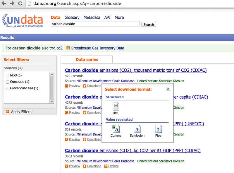
So let's write a simple scraper to grab the results and see if you can download a selected ata file automatically...
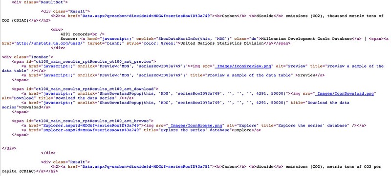
If we View Source on the results page we can look for the individual results items - and see what we neeed to parse out.
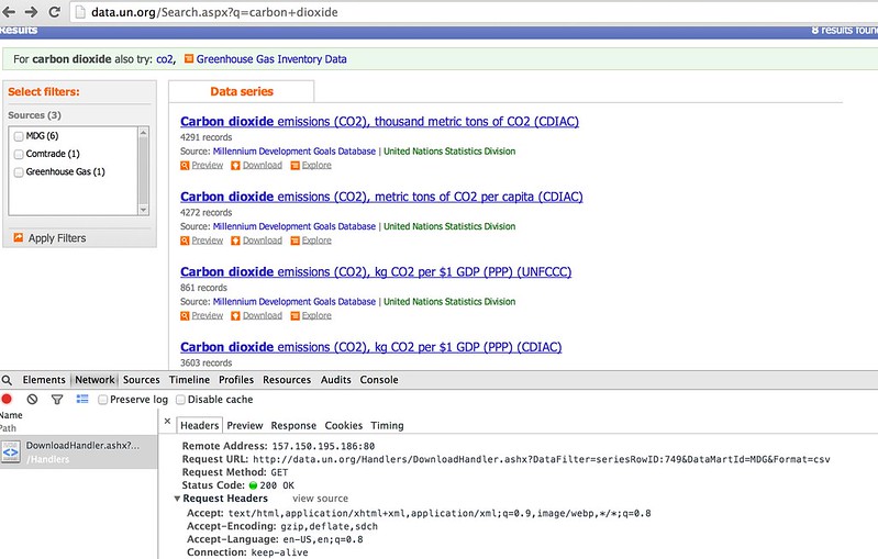
We also need to have a look at what form the HTTP request for a data download looks like to make sure we get what we need when we do scrape the results...
#Load in some libraries to handle the web page requests and the web page parsing...
import requests
from bs4 import BeautifulSoup

#Note - I'm in Python3
from urllib.parse import parse_qs

#The scraper will be limited to just the first results page...
def searchUNdata(q):
    ''' Run a search on the UN data website and scrape the results '''

    params={'q':q}
    url='http://data.un.org/Search.aspx'

    response = requests.get(url,params=params)

    soup=BeautifulSoup(response.content)

    results={}

    #Get the list of results
    searchresults=soup.findAll('div',{'class':'Result'})

    #For each result, parse out the name of the dataset, the datamart ID and the data filter ID
    for result in searchresults:
        h2=result.find('h2')
        #We can find everything we need in the <a> tag...
        a=h2.find('a')
        p=parse_qs(a.attrs['href'])
        results[a.text]=(p['d'][0],p['f'][0])

    return results
#A couple of helper functions to let us display the results

results=searchUNdata('carbon dioxide')

def printResults(results):
    ''' Nicely print the search results '''

    for result in results.keys():
        print(result)


def unDataSearch(q):
    ''' Simple function to take a searh phrase, run the search on the UN data site, and print and return the results. '''

    results=searchUNdata(q)
    printResults(results)
    return results

printResults(results)

#q='carbon dioxide'
#unDataSearch(q)
Carbon dioxide emissions (CO2), thousand metric tons of CO2 (CDIAC)
Carbon dioxide (CO2) Emissions without Land Use, Land-Use Change and Forestry (LULUCF), in Gigagrams (Gg)
Carbon dioxide emissions (CO2), kg CO2 per $1 GDP (PPP) (CDIAC)
Carbon dioxide emissions (CO2), metric tons of CO2 per capita (UNFCCC)
Trade of goods , US$, HS 1992, 28 Inorganic chemicals, precious metal compound, isotope
Carbon dioxide emissions (CO2), kg CO2 per $1 GDP (PPP) (UNFCCC)
Carbon dioxide emissions (CO2), thousand metric tons of CO2 (UNFCCC)
Carbon dioxide emissions (CO2), metric tons of CO2 per capita (CDIAC)
#Just in case - a helper routine for working with the search results data
def search(d, substr):
    ''' Partial string match search within dict key names '''
    #via http://stackoverflow.com/a/10796050/454773

    result = []
    for key in d:
        if substr.lower() in key.lower():
            result.append((key, d[key]))

    return result
search(results, 'per capita')
[('Carbon dioxide emissions (CO2), metric tons of CO2 per capita (UNFCCC)',
  ('MDG', 'seriesRowID:752')),
 ('Carbon dioxide emissions (CO2), metric tons of CO2 per capita (CDIAC)',
  ('MDG', 'seriesRowID:751'))]
#Note - I'm in Python3
from io import BytesIO

import zipfile
import pandas as pd

def getUNdata(undataSearchResults,dataset):
    ''' Download a named dataset from the UN Data website and load it into a pandas dataframe '''

    datamartID,seriesRowID=undataSearchResults[dataset]

    url='http://data.un.org/Handlers/DownloadHandler.ashx?DataFilter='+seriesRowID+'&DataMartId='+datamartID+'&Format=csv'

    r = requests.get(url)


    s=BytesIO(r.content)
    z = zipfile.ZipFile(s)

    #Show the files in the zip file
    #z.namelist()

    #Let's assume we just get one file per zip...
    #Drop any all blank columns
    df=pd.read_csv( BytesIO( z.read( z.namelist()[0] ) )).dropna(axis=1,how='all')
    return df
results=unDataSearch('carbon dioxide')
Carbon dioxide emissions (CO2), thousand metric tons of CO2 (CDIAC)
Carbon dioxide (CO2) Emissions without Land Use, Land-Use Change and Forestry (LULUCF), in Gigagrams (Gg)
Carbon dioxide emissions (CO2), kg CO2 per $1 GDP (PPP) (CDIAC)
Carbon dioxide emissions (CO2), metric tons of CO2 per capita (UNFCCC)
Trade of goods , US$, HS 1992, 28 Inorganic chemicals, precious metal compound, isotope
Carbon dioxide emissions (CO2), kg CO2 per $1 GDP (PPP) (UNFCCC)
Carbon dioxide emissions (CO2), thousand metric tons of CO2 (UNFCCC)
Carbon dioxide emissions (CO2), metric tons of CO2 per capita (CDIAC)
dd=getUNdata(results,'Carbon dioxide emissions (CO2), metric tons of CO2 per capita (UNFCCC)')
dd
| Country or Area | Year | Value | Value Footnotes | Value Footnotes.1 | |
|---|---|---|---|---|---|
| 0 | Australia | 2010 | 18.042955 | NaN | NaN |
| 1 | Australia | 2009 | 18.394162 | NaN | NaN |
| 2 | Australia | 2008 | 18.680381 | NaN | NaN |
| 3 | Australia | 2007 | 18.700552 | NaN | NaN |
| 4 | Australia | 2006 | 18.660320 | NaN | NaN |
| 5 | Australia | 2005 | 18.741587 | NaN | NaN |
| 6 | Australia | 2004 | 18.887782 | NaN | NaN |
| 7 | Australia | 2003 | 18.833971 | NaN | NaN |
| 8 | Australia | 2002 | 18.382553 | NaN | NaN |
| 9 | Australia | 2001 | 18.369852 | NaN | NaN |
| 10 | Australia | 2000 | 18.249353 | NaN | NaN |
| 11 | Australia | 1999 | 18.110541 | NaN | NaN |
| 12 | Australia | 1998 | 17.790195 | NaN | NaN |
| 13 | Australia | 1997 | 17.276190 | NaN | NaN |
| 14 | Australia | 1996 | 17.017798 | NaN | NaN |
| 15 | Australia | 1995 | 16.791157 | NaN | NaN |
| 16 | Australia | 1994 | 16.382401 | NaN | NaN |
| 17 | Australia | 1993 | 16.292707 | NaN | NaN |
| 18 | Australia | 1992 | 16.247799 | NaN | NaN |
| 19 | Australia | 1991 | 16.145272 | NaN | NaN |
| 20 | Australia | 1990 | 16.274010 | NaN | NaN |
| 21 | Austria | 2010 | 8.612525 | NaN | NaN |
| 22 | Austria | 2009 | 8.032090 | NaN | NaN |
| 23 | Austria | 2008 | 8.861574 | NaN | NaN |
| 24 | Austria | 2007 | 8.948816 | NaN | NaN |
| 25 | Austria | 2006 | 9.311083 | NaN | NaN |
| 26 | Austria | 2005 | 9.684401 | NaN | NaN |
| 27 | Austria | 2004 | 9.555359 | NaN | NaN |
| 28 | Austria | 2003 | 9.559380 | NaN | NaN |
| 29 | Austria | 2002 | 8.872889 | NaN | NaN |
| ... | ... | ... | ... | ... | ... |
| 834 | United Kingdom | 1995 | 9.525717 | 1 | 1 |
| 835 | United Kingdom | 1994 | 9.695512 | 1 | 1 |
| 836 | United Kingdom | 1993 | 9.824330 | 1 | 1 |
| 837 | United Kingdom | 1992 | 10.087042 | 1 | 1 |
| 838 | United Kingdom | 1991 | 10.399337 | 1 | 1 |
| 839 | United Kingdom | 1990 | 10.301924 | 1 | 1 |
| 840 | United States | 2010 | 18.115315 | 1 | 1 |
| 841 | United States | 2009 | 17.613975 | 1 | 1 |
| 842 | United States | 2008 | 19.134200 | 1 | 1 |
| 843 | United States | 2007 | 19.938306 | 1 | 1 |
| 844 | United States | 2006 | 19.790435 | 1 | 1 |
| 845 | United States | 2005 | 20.264177 | 1 | 1 |
| 846 | United States | 2004 | 20.319687 | 1 | 1 |
| 847 | United States | 2003 | 20.138513 | 1 | 1 |
| 848 | United States | 2002 | 20.141864 | 1 | 1 |
| 849 | United States | 2001 | 20.227848 | 1 | 1 |
| 850 | United States | 2000 | 20.813767 | 1 | 1 |
| 851 | United States | 1999 | 20.421978 | 1 | 1 |
| 852 | United States | 1998 | 20.371008 | 1 | 1 |
| 853 | United States | 1997 | 20.500903 | 1 | 1 |
| 854 | United States | 1996 | 20.458236 | 1 | 1 |
| 855 | United States | 1995 | 20.023986 | 1 | 1 |
| 856 | United States | 1994 | 19.986553 | 1 | 1 |
| 857 | United States | 1993 | 19.879693 | 1 | 1 |
| 858 | United States | 1992 | 19.647320 | 1 | 1 |
| 859 | United States | 1991 | 19.437409 | 1 | 1 |
| 860 | United States | 1990 | 19.801924 | 1 | 1 |
| 861 | NaN | NaN | NaN | NaN | NaN |
| 862 | footnoteSeqID | Footnote | NaN | NaN | NaN |
| 863 | 1 | For Denmark, France, United Kingdom and United... | NaN | NaN | NaN |
864 rows × 5 columns
#One thing to note is that footnotes may appear at the bottom of a dataframe
#We can spot the all empty row and drop rows from that
#We can also drop the footnote related columns
def dropFootnotes(df):
    return df[:pd.isnull(dd).all(1).nonzero()[0][0]].drop(['Value Footnotes','Value Footnotes.1'], 1)

dropFootnotes(dd)
| Country or Area | Year | Value | |
|---|---|---|---|
| 0 | Australia | 2010 | 18.042955 |
| 1 | Australia | 2009 | 18.394162 |
| 2 | Australia | 2008 | 18.680381 |
| 3 | Australia | 2007 | 18.700552 |
| 4 | Australia | 2006 | 18.660320 |
| 5 | Australia | 2005 | 18.741587 |
| 6 | Australia | 2004 | 18.887782 |
| 7 | Australia | 2003 | 18.833971 |
| 8 | Australia | 2002 | 18.382553 |
| 9 | Australia | 2001 | 18.369852 |
| 10 | Australia | 2000 | 18.249353 |
| 11 | Australia | 1999 | 18.110541 |
| 12 | Australia | 1998 | 17.790195 |
| 13 | Australia | 1997 | 17.276190 |
| 14 | Australia | 1996 | 17.017798 |
| 15 | Australia | 1995 | 16.791157 |
| 16 | Australia | 1994 | 16.382401 |
| 17 | Australia | 1993 | 16.292707 |
| 18 | Australia | 1992 | 16.247799 |
| 19 | Australia | 1991 | 16.145272 |
| 20 | Australia | 1990 | 16.274010 |
| 21 | Austria | 2010 | 8.612525 |
| 22 | Austria | 2009 | 8.032090 |
| 23 | Austria | 2008 | 8.861574 |
| 24 | Austria | 2007 | 8.948816 |
| 25 | Austria | 2006 | 9.311083 |
| 26 | Austria | 2005 | 9.684401 |
| 27 | Austria | 2004 | 9.555359 |
| 28 | Austria | 2003 | 9.559380 |
| 29 | Austria | 2002 | 8.872889 |
| ... | ... | ... | ... |
| 831 | United Kingdom | 1998 | 9.480194 |
| 832 | United Kingdom | 1997 | 9.435972 |
| 833 | United Kingdom | 1996 | 9.877613 |
| 834 | United Kingdom | 1995 | 9.525717 |
| 835 | United Kingdom | 1994 | 9.695512 |
| 836 | United Kingdom | 1993 | 9.824330 |
| 837 | United Kingdom | 1992 | 10.087042 |
| 838 | United Kingdom | 1991 | 10.399337 |
| 839 | United Kingdom | 1990 | 10.301924 |
| 840 | United States | 2010 | 18.115315 |
| 841 | United States | 2009 | 17.613975 |
| 842 | United States | 2008 | 19.134200 |
| 843 | United States | 2007 | 19.938306 |
| 844 | United States | 2006 | 19.790435 |
| 845 | United States | 2005 | 20.264177 |
| 846 | United States | 2004 | 20.319687 |
| 847 | United States | 2003 | 20.138513 |
| 848 | United States | 2002 | 20.141864 |
| 849 | United States | 2001 | 20.227848 |
| 850 | United States | 2000 | 20.813767 |
| 851 | United States | 1999 | 20.421978 |
| 852 | United States | 1998 | 20.371008 |
| 853 | United States | 1997 | 20.500903 |
| 854 | United States | 1996 | 20.458236 |
| 855 | United States | 1995 | 20.023986 |
| 856 | United States | 1994 | 19.986553 |
| 857 | United States | 1993 | 19.879693 |
| 858 | United States | 1992 | 19.647320 |
| 859 | United States | 1991 | 19.437409 |
| 860 | United States | 1990 | 19.801924 |
861 rows × 3 columns
Summary
This notebook demonstrates a simple, informal scraper based API to the UN data website. Searches can be run on the UN data website to obtain a list of named datasets, and then a specified named dataset can be automatically downloaded into a pandas dataframe.