Notebook

In [224]:

import numpy as np
%matplotlib inline

Shocktube: shock with specified Mach number¶

Here we set up a shock tube with specified right state

$[\rho_r, u_r=0, p_r]$

and left velocity $u_l=0$ , such that the solution consists of a right-going shock wave moving at a prescribed Mach number $M$ relative to the right ambient state:

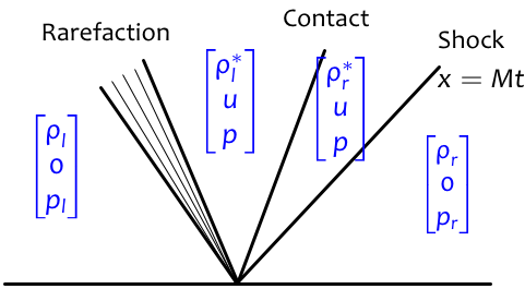
$s = M c_r.$

What we know in advance about the Riemann solution is depicted below.

Let

$\mu = \frac{2(M^2-1)}{M(\gamma+1)}.$

Using the Rankine-Hugoniot conditions, we find that the state just to the right of the contact is given by the following:

$\begin{align} \rho_r^*& = \rho_r \frac{M}{M-\mu} \\ u & = \mu c_r \\ p & = p_r \frac{(2M^2 -1)\gamma+1}{\gamma+1}. \end{align}$

Next, we know that the left state and the $[\rho_l^*, u, p]$ state must be connected by a left-going rarefaction. The relevant Riemann invariants imply

$\rho_l = \frac{4\gamma p_l}{(\gamma-1)^2 u^2} \left(1- \left(\frac{p}{p_l}\right)^{\frac{\gamma-1}{2\gamma}}\right)^2$

and

$\rho_l^* = \left(\frac{p}{p_l}\right)^{1/\gamma} \rho_l.$

So we can prescribe any value we like for $p_l$ and compute the remaining values $\rho_l,\rho_l^*$ from the equations above. The only catch is that the resulting rarefaction should satisfy the entropy condition, which is true if $p_l>p$ .

In [225]:

gamma = 1.4
M = 1.5

# Right state
rho_r = 1.0
u_r   = 0.0  # This must be zero.
p_r   = 1.0

# Left state
p_l   = 5.0
u_l   = 0.0    # This must be zero.

In [226]:

c_r = np.sqrt(gamma*p_r/rho_r)  # Right state sound speed
s = M * c_r                     # Shock speed
mu = 2*(M**2-1)/(gamma+1)/M

# Find state to right of discontinuity via Rankine-Hugoniot conditions
p   = p_r * ((2*M**2-1)*gamma+1)/(gamma+1)
u   = mu*c_r
rho_rs = rho_r*M/(M-mu)

# Check that the 1-wave is a rarefaction
if p_l<p:
    print "Warning: the states provided do not lead to the expected solution structure."

In [227]:

# Find remaining densities
rho_l = 4*gamma*p_l/((gamma-1)**2*u**2) * (1-(p/p_l)**((gamma-1)/(2*gamma)))**2
rho_ls= (p/p_l)**(1/gamma) * rho_l

In [228]:

from clawpack import pyclaw
from clawpack import riemann
from clawpack.riemann.euler_with_efix_1D_constants import density, momentum, energy, num_eqn

In [229]:

# Specify equations and boundary conditions
solver = pyclaw.ClawSolver1D(riemann.euler_with_efix_1D)
solver.bc_lower[0] = pyclaw.BC.extrap
solver.bc_upper[0] = pyclaw.BC.extrap

In [230]:

# Grid
x = pyclaw.Dimension('x',-1.,1.,1000)
domain = pyclaw.Domain([x])
state = pyclaw.State(domain,num_eqn)
state.problem_data['gamma'] = gamma
xc = state.grid.p_centers[0]

In [231]:

# Initial values
state.q[density,:] = rho_l*(xc<0) + rho_r*(xc>=0)
state.q[momentum,:] = rho_l*u_l*(xc<0) + rho_r*u_r*(xc>=0)
E_r = 0.5*rho_r * u_r**2 + p_r/(gamma-1)
E_l = 0.5*rho_l * u_l**2 + p_l/(gamma-1)
state.q[energy, :] = E_l*(xc<0) + E_r*(xc>=0)

In [232]:

claw = pyclaw.Controller()
claw.tfinal = 1.
claw.solution = pyclaw.Solution(state,domain)
claw.solver = solver
claw.num_output_times = 10
claw.keep_copy = True

In [233]:

claw.run()

2014-10-20 14:07:29,134 INFO CLAW: Solution 0 computed for time t=0.000000
2014-10-20 14:07:29,193 INFO CLAW: Solution 1 computed for time t=0.100000
2014-10-20 14:07:29,256 INFO CLAW: Solution 2 computed for time t=0.200000
2014-10-20 14:07:29,332 INFO CLAW: Solution 3 computed for time t=0.300000
2014-10-20 14:07:29,421 INFO CLAW: Solution 4 computed for time t=0.400000
2014-10-20 14:07:29,497 INFO CLAW: Solution 5 computed for time t=0.500000
2014-10-20 14:07:29,562 INFO CLAW: Solution 6 computed for time t=0.600000
2014-10-20 14:07:29,628 INFO CLAW: Solution 7 computed for time t=0.700000
2014-10-20 14:07:29,694 INFO CLAW: Solution 8 computed for time t=0.800000
2014-10-20 14:07:29,759 INFO CLAW: Solution 9 computed for time t=0.900000
2014-10-20 14:07:29,824 INFO CLAW: Solution 10 computed for time t=1.000000

Out[233]:

{'cflmax': 0.953655319923049,
 'dtmax': 0.0010564183672772706,
 'dtmin': 0.0007603515077312271,
 'numsteps': 1319}

In [234]:

from matplotlib import animation
from clawpack.visclaw.JSAnimation import IPython_display
import matplotlib.pyplot as plt

In [236]:

# Animated plot of the solution density
fig = plt.figure(figsize=[8,4])
ymax = max(rho_l, rho_ls, rho_rs, rho_r)
ax = plt.axes(xlim=(xc[0], xc[-1]), ylim=(0, ymax+0.5))
line, = ax.plot([], [], lw=1)

def fplot(i):
    frame = claw.frames[i]
    q = frame.q[0,:]
    line.set_data(xc, q)
    ax.set_title('Density at t= '+ str(frame.t))
    return line,

animation.FuncAnimation(fig, fplot, frames=len(claw.frames))

Out[236]:

In [235]: