Notes on Neural Networks and Deep Learning, chapter 1
This notebook collects notes and code from Chapter 1 of Neural Networks and Deep Learning, chapter 1.
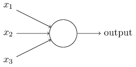
Foundations: Perceptron
A perceptron simply takes a weighted combination of its inputs and outputs a binary 1 or 0 when this combination is larger than some threshold: output={1Wx+b≤00Wx+b>0
The Neural Network
A straightforward extension of the perceptron is to create a network of layers of perceptrons (or units), where units from one layer are connected to units in the next:
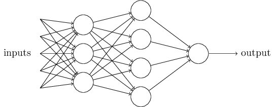
In this setting, the mixing weights for each layer become a matrix W∈Rm×n and the threshold (or bias) becomes a vector b∈Rm, where n is the number of inputs to a layer and m is the number of outputs.
One additional deviation from the original perceptron is that in practice we typically use a logistic function instead of a hard threshold. That is, instead of switching immediately between 0 and 1, we use a function which transitions between the two values smoothly. This is so that a small change in the W or b doesn't cause a large change in the output when Wx+b is close to 0, or in other words, so that the network function is differentiable. A common choise is the logistic sigmoid: σ(z)=11+e−z
Notation
We'll use the following notation:
L - Number of layers in the network.
Nn - Dimensionality of layer n∈{0,…,L}. N0 is the dimensionality of the input; NL is the dimensionality of the output.
Wm∈RNm×Nm−1 - Weight matrix for layer m∈{1,…,L}. Wmij is the weight between the ith unit in layer m and the jth unit in layer m−1.
bm∈RNm - Bias vector for layer m.
σm - Nonlinear activation function of the units in layer m, applied elementwise.
zm∈RNm - Linear mix of the inputs to layer m, computed by zm=Wmam−1+bm.
am∈RNm - Activation of units in layer m, computed by am=σm(hm)=σm(Wmam−1+bm). aL is the output of the network. We define the special case a0 as the input of the network.
y∈RNL - Target output of the network.
C - Cost/error function of the network, which is a function of aL (the network output) and y (treated as a constant).
Training a Neural Network with Gradient Descent
In a typical setting, we want our neural network to be able to predict an output given some input based on some training data of input-output pairs x,y. An example used here is to predict the numerical value of a digital image of a handwritten digit. To do so, we first define a cost function: C=12n∑x||y−aL||2
The most common method for minimizing the cost function is to use gradient descent. Gradient descent simply adjusts the parameters Wm and bm in a direction opposite of the gradient of the cost function, which is guaranteed to decrease the value of the cost function. To do so, we need to know the gradient of C with respect Wm and bm which is computed by backpropagation (not covered here). That is, gradient descent updates the parameters by Wm′=Wm−η∂C∂Wm
Example: Training a Neural Network to classify MNIST
The following code trains a neural network with sigmoid acivation function using gradient descent to classify the MNIST dataset.
import numpy as np
import random
import cPickle
import gzip
import theano
import theano.tensor as T
import matplotlib.pyplot as plt
%matplotlib inline
def load_data():
    """Return the MNIST data as a tuple containing the training data,
    the validation data, and the test data.

    The ``training_data`` is returned as a tuple with two entries.
    The first entry contains the actual training images.  This is a
    numpy ndarray with 50,000 entries.  Each entry is, in turn, a
    numpy ndarray with 784 values, representing the 28 * 28 = 784
    pixels in a single MNIST image.

    The second entry in the ``training_data`` tuple is a numpy ndarray
    containing 50,000 entries.  Those entries are just the digit
    values (0...9) for the corresponding images contained in the first
    entry of the tuple.

    The ``validation_data`` and ``test_data`` are similar, except
    each contains only 10,000 images.

    This is a nice data format, but for use in neural networks it's
    helpful to modify the format of the ``training_data`` a little.
    That's done in the wrapper function ``load_data_wrapper()``, see
    below.
    """
    f = gzip.open('mnist.pkl.gz', 'rb')
    training_data, validation_data, test_data = cPickle.load(f)
    f.close()
    return (training_data, validation_data, test_data)

def load_data_wrapper():
    """Return a tuple containing ``(training_data, validation_data,
    test_data)``. Based on ``load_data``, but the format is more
    convenient for use in our implementation of neural networks.

    In particular, ``training_data`` is a list containing 50,000
    2-tuples ``(x, y)``.  ``x`` is a 784-dimensional numpy.ndarray
    containing the input image.  ``y`` is a 10-dimensional
    numpy.ndarray representing the unit vector corresponding to the
    correct digit for ``x``.

    ``validation_data`` and ``test_data`` are lists containing 10,000
    2-tuples ``(x, y)``.  In each case, ``x`` is a 784-dimensional
    numpy.ndarry containing the input image, and ``y`` is the
    corresponding classification, i.e., the digit values (integers)
    corresponding to ``x``.

    Obviously, this means we're using slightly different formats for
    the training data and the validation / test data.  These formats
    turn out to be the most convenient for use in our neural network
    code."""
    tr_d, va_d, te_d = load_data()
    training_inputs = [np.reshape(x, (784, 1)) for x in tr_d[0]]
    training_results = [vectorized_result(y) for y in tr_d[1]]
    training_data = zip(training_inputs, training_results)
    validation_inputs = [np.reshape(x, (784, 1)) for x in va_d[0]]
    validation_data = zip(validation_inputs, va_d[1])
    test_inputs = [np.reshape(x, (784, 1)) for x in te_d[0]]
    test_data = zip(test_inputs, te_d[1])
    return (training_data, validation_data, test_data)

def vectorized_result(j):
    """Return a 10-dimensional unit vector with a 1.0 in the jth
    position and zeroes elsewhere.  This is used to convert a digit
    (0...9) into a corresponding desired output from the neural
    network."""
    e = np.zeros((10, 1))
    e[j] = 1.0
    return e
class Network():

    def __init__(self, sizes):
        """The list ``sizes`` contains the number of neurons in the
        respective layers of the network.  For example, if the list
        was [2, 3, 1] then it would be a three-layer network, with the
        first layer containing 2 neurons, the second layer 3 neurons,
        and the third layer 1 neuron.  The biases and weights for the
        network are initialized randomly, using a Gaussian
        distribution with mean 0, and variance 1.  Note that the first
        layer is assumed to be an input layer, and by convention we
        won't set any biases for those neurons, since biases are only
        ever used in computing the outputs from later layers."""
        self.num_layers = len(sizes)
        self.sizes = sizes
        self.biases = [np.random.randn(y, 1) for y in sizes[1:]]
        self.weights = [np.random.randn(y, x)
                        for x, y in zip(sizes[:-1], sizes[1:])]

    def feedforward(self, a):
        """Return the output of the network if ``a`` is input."""
        for b, w in zip(self.biases, self.weights):
            a = sigmoid_vec(np.dot(w, a)+b)
        return a

    def SGD(self, training_data, epochs, mini_batch_size, eta,
            test_data=None):
        """Train the neural network using mini-batch stochastic
        gradient descent.  The ``training_data`` is a list of tuples
        ``(x, y)`` representing the training inputs and the desired
        outputs.  The other non-optional parameters are
        self-explanatory.  If ``test_data`` is provided then the
        network will be evaluated against the test data after each
        epoch, and partial progress printed out.  This is useful for
        tracking progress, but slows things down substantially."""
        if test_data: n_test = len(test_data)
        n = len(training_data)
        for j in xrange(epochs):
            random.shuffle(training_data)
            mini_batches = [
                training_data[k:k+mini_batch_size]
                for k in xrange(0, n, mini_batch_size)]
            for mini_batch in mini_batches:
                self.update_mini_batch(mini_batch, eta)
            if test_data:
                print "Epoch {0}: {1} / {2}".format(
                    j, self.evaluate(test_data), n_test)
            else:
                print "Epoch {0} complete".format(j)

    def update_mini_batch(self, mini_batch, eta):
        """Update the network's weights and biases by applying
        gradient descent using backpropagation to a single mini batch.
        The ``mini_batch`` is a list of tuples ``(x, y)``, and ``eta``
        is the learning rate."""
        nabla_b = [np.zeros(b.shape) for b in self.biases]
        nabla_w = [np.zeros(w.shape) for w in self.weights]
        for x, y in mini_batch:
            delta_nabla_b, delta_nabla_w = self.backprop(x, y)
            nabla_b = [nb+dnb for nb, dnb in zip(nabla_b, delta_nabla_b)]
            nabla_w = [nw+dnw for nw, dnw in zip(nabla_w, delta_nabla_w)]
        self.weights = [w-(eta/len(mini_batch))*nw
                        for w, nw in zip(self.weights, nabla_w)]
        self.biases = [b-(eta/len(mini_batch))*nb
                       for b, nb in zip(self.biases, nabla_b)]

    def backprop(self, x, y):
        """Return a tuple ``(nabla_b, nabla_w)`` representing the
        gradient for the cost function C_x.  ``nabla_b`` and
        ``nabla_w`` are layer-by-layer lists of numpy arrays, similar
        to ``self.biases`` and ``self.weights``."""
        nabla_b = [np.zeros(b.shape) for b in self.biases]
        nabla_w = [np.zeros(w.shape) for w in self.weights]
        # feedforward
        activation = x
        activations = [x] # list to store all the activations, layer by layer
        zs = [] # list to store all the z vectors, layer by layer
        for b, w in zip(self.biases, self.weights):
            z = np.dot(w, activation)+b
            zs.append(z)
            activation = sigmoid_vec(z)
            activations.append(activation)
        # backward pass
        delta = self.cost_derivative(activations[-1], y) * \
            sigmoid_prime_vec(zs[-1])
        nabla_b[-1] = delta
        nabla_w[-1] = np.dot(delta, activations[-2].transpose())
        # Note that the variable l in the loop below is used a little
        # differently to the notation in Chapter 2 of the book.  Here,
        # l = 1 means the last layer of neurons, l = 2 is the
        # second-last layer, and so on.  It's a renumbering of the
        # scheme in the book, used here to take advantage of the fact
        # that Python can use negative indices in lists.
        for l in xrange(2, self.num_layers):
            z = zs[-l]
            spv = sigmoid_prime_vec(z)
            delta = np.dot(self.weights[-l+1].transpose(), delta) * spv
            nabla_b[-l] = delta
            nabla_w[-l] = np.dot(delta, activations[-l-1].transpose())
        return (nabla_b, nabla_w)

    def evaluate(self, test_data):
        """Return the number of test inputs for which the neural
        network outputs the correct result. Note that the neural
        network's output is assumed to be the index of whichever
        neuron in the final layer has the highest activation."""
        test_results = [(np.argmax(self.feedforward(x)), y)
                        for (x, y) in test_data]
        return sum(int(x == y) for (x, y) in test_results)

    def cost_derivative(self, output_activations, y):
        """Return the vector of partial derivatives \partial C_x /
        \partial a for the output activations."""
        return (output_activations-y)

#### Miscellaneous functions
def sigmoid(z):
    """The sigmoid function."""
    return 1.0/(1.0+np.exp(-z))

sigmoid_vec = np.vectorize(sigmoid)

def sigmoid_prime(z):
    """Derivative of the sigmoid function."""
    return sigmoid(z)*(1-sigmoid(z))

sigmoid_prime_vec = np.vectorize(sigmoid_prime)
training_data, validation_data, test_data = load_data_wrapper()
# Plot a few example training digits
plt.figure(figsize=(6, 6))
for n in range(9):
    plt.subplot(3, 3, n)
    plt.imshow(training_data[n][0].reshape(28, 28), interpolation='nearest', cmap=plt.cm.gray_r)
    plt.axis('off')
    plt.title(np.argmax(training_data[n][1]))

# Initialize the network
net = Network([784, 30, 10])
# Training for 10 epochs using a mini-batch size of 10, with a learning rate of 3.
net.SGD(training_data, 10, 10, 3.0, test_data=test_data)
Epoch 0: 9067 / 10000
Epoch 1: 9202 / 10000
Epoch 2: 9283 / 10000
Epoch 3: 9318 / 10000
Epoch 4: 9376 / 10000
Epoch 5: 9393 / 10000
Epoch 6: 9399 / 10000
Epoch 7: 9426 / 10000
Epoch 8: 9443 / 10000
Epoch 9: 9454 / 10000
Using Theano
For completeness, here's an implementation of the above using Theano based on my Theano tutorial.
class Layer(object):
    def __init__(self, W_init, b_init, activation):
        '''
        A layer of a neural network, computes s(Wx + b) where s is a nonlinearity and x is the input vector.

        :parameters:
            - W_init : np.ndarray, shape=(n_output, n_input)
                Values to initialize the weight matrix to.
            - b_init : np.ndarray, shape=(n_output,)
                Values to initialize the bias vector
            - activation : theano.tensor.elemwise.Elemwise
                Activation function for layer output
        '''
        # Retrieve the input and output dimensionality based on W's initialization
        n_output, n_input = W_init.shape
        # Make sure b is n_output in size
        assert b_init.shape == (n_output,)
        # All parameters should be shared variables.
        # They're used in this class to compute the layer output,
        # but are updated elsewhere when optimizing the network parameters.
        # Note that we are explicitly requiring that W_init has the theano.config.floatX dtype
        self.W = theano.shared(value=W_init.astype(theano.config.floatX),
                               # The name parameter is solely for printing purporses
                               name='W',
                               # Setting borrow=True allows Theano to use user memory for this object.
                               # It can make code slightly faster by avoiding a deep copy on construction.
                               # For more details, see
                               # http://deeplearning.net/software/theano/tutorial/aliasing.html
                               borrow=True)
        # We can force our bias vector b to be a column vector using numpy's reshape method.
        # When b is a column vector, we can pass a matrix-shaped input to the layer
        # and get a matrix-shaped output, thanks to broadcasting (described below)
        self.b = theano.shared(value=b_init.reshape(-1, 1).astype(theano.config.floatX),
                               name='b',
                               borrow=True,
                               # Theano allows for broadcasting, similar to numpy.
                               # However, you need to explicitly denote which axes can be broadcasted.
                               # By setting broadcastable=(False, True), we are denoting that b
                               # can be broadcast (copied) along its second dimension in order to be
                               # added to another variable.  For more information, see
                               # http://deeplearning.net/software/theano/library/tensor/basic.html
                               broadcastable=(False, True))
        self.activation = activation
        # We'll compute the gradient of the cost of the network with respect to the parameters in this list.
        self.params = [self.W, self.b]

    def output(self, x):
        '''
        Compute this layer's output given an input

        :parameters:
            - x : theano.tensor.var.TensorVariable
                Theano symbolic variable for layer input

        :returns:
            - output : theano.tensor.var.TensorVariable
                Mixed, biased, and activated x
        '''
        # Compute linear mix
        lin_output = T.dot(self.W, x) + self.b
        # Output is just linear mix if no activation function
        # Otherwise, apply the activation function
        return (lin_output if self.activation is None else self.activation(lin_output))

class MLP(object):
    def __init__(self, W_init, b_init, activations):
        '''
        Multi-layer perceptron class, computes the composition of a sequence of Layers

        :parameters:
            - W_init : list of np.ndarray, len=N
                Values to initialize the weight matrix in each layer to.
                The layer sizes will be inferred from the shape of each matrix in W_init
            - b_init : list of np.ndarray, len=N
                Values to initialize the bias vector in each layer to
            - activations : list of theano.tensor.elemwise.Elemwise, len=N
                Activation function for layer output for each layer
        '''
        # Make sure the input lists are all of the same length
        assert len(W_init) == len(b_init) == len(activations)

        # Initialize lists of layers
        self.layers = []
        # Construct the layers
        for W, b, activation in zip(W_init, b_init, activations):
            self.layers.append(Layer(W, b, activation))

        # Combine parameters from all layers
        self.params = []
        for layer in self.layers:
            self.params += layer.params

    def output(self, x):
        '''
        Compute the MLP's output given an input

        :parameters:
            - x : theano.tensor.var.TensorVariable
                Theano symbolic variable for network input

        :returns:
            - output : theano.tensor.var.TensorVariable
                x passed through the MLP
        '''
        # Recursively compute output
        for layer in self.layers:
            x = layer.output(x)
        return x

    def squared_error(self, x, y):
        '''
        Compute the squared euclidean error of the network output against the "true" output y

        :parameters:
            - x : theano.tensor.var.TensorVariable
                Theano symbolic variable for network input
            - y : theano.tensor.var.TensorVariable
                Theano symbolic variable for desired network output

        :returns:
            - error : theano.tensor.var.TensorVariable
                The squared Euclidian distance between the network output and y
        '''
        return T.sum((self.output(x) - y)**2)

def gradient_updates(cost, params, learning_rate):
    '''
    Compute updates for gradient descent

    :parameters:
        - cost : theano.tensor.var.TensorVariable
            Theano cost function to minimize
        - params : list of theano.tensor.var.TensorVariable
            Parameters to compute gradient against
        - learning_rate : float
            Gradient descent learning rate

    :returns:
        updates : list
            List of updates, one for each parameter
    '''
    # List of update steps for each parameter
    updates = []
    # Just gradient descent on cost
    for param in params:
        # Each parameter is updated by taking a step in the opposite direction of the gradient.
        updates.append((param, param - learning_rate*T.grad(cost, param)))
    return updates
# First, set the size of each layer (and the number of layers)
# Input layer size is training data dimensionality - 28*28 = 784
# Output size is target dimensionality, here 1 of 10 digits, so size = 10
# Finally, let the hidden layer have 30 neurons as above.
# If we wanted more layers, we could just add another layer size to this list.
layer_sizes = [training_data[0][0].shape[0], 30, training_data[0][1].shape[0]]
# Set initial parameter values
W_init = []
b_init = []
activations = []
for n_input, n_output in zip(layer_sizes[:-1], layer_sizes[1:]):
    # Getting the correct initialization matters a lot for non-toy problems.
    # However, here we can just use the following initialization with success:
    # Normally distribute initial weights
    W_init.append(np.random.randn(n_output, n_input))
    # Set initial biases to 1
    b_init.append(np.ones(n_output))
    # We'll use sigmoid activation for all layers
    # Note that this doesn't make a ton of sense when using squared distance
    # because the sigmoid function is bounded on [0, 1].
    activations.append(T.nnet.sigmoid)
# Create an instance of the MLP class
mlp = MLP(W_init, b_init, activations)
# Create Theano variables for the MLP input
mlp_input = T.matrix('mlp_input')
# ... and the desired output
mlp_target = T.matrix('mlp_target')
# Number of examples in each mini-batch
batch_size = 10
# Learning rate is 3., but our MLP doesn't normalize by batch size so we do it here
learning_rate = 3./batch_size
# Create a function for computing the cost of the network given an input
cost = mlp.squared_error(mlp_input, mlp_target)
# Create a theano function for training the network
train = theano.function([mlp_input, mlp_target], cost,
                        updates=gradient_updates(cost, mlp.params, learning_rate))
# Create a theano function for computing the MLP's output given some input
mlp_output = theano.function([mlp_input], mlp.output(mlp_input))
# Number of times to iterate over the training set
n_epochs = 10
for epoch in range(n_epochs):
    random.shuffle(training_data)
    mini_batches = [training_data[k:k+batch_size] for k in xrange(0, len(training_data), batch_size)]
    for mini_batch in mini_batches:
        train(np.hstack(X[0] for X in mini_batch), np.hstack(X[1] for X in mini_batch))
    test_output = mlp_output(np.hstack([X[0] for X in test_data]))
    n_correct = np.sum(np.argmax(test_output, axis=0) == [X[1] for X in test_data])
    print "Epoch {0}: {1} / {2}".format(epoch, n_correct, len(test_data))
Epoch 0: 9095 / 10000
Epoch 1: 9270 / 10000
Epoch 2: 9317 / 10000
Epoch 3: 9313 / 10000
Epoch 4: 9355 / 10000
Epoch 5: 9403 / 10000
Epoch 6: 9413 / 10000
Epoch 7: 9397 / 10000
Epoch 8: 9360 / 10000
Epoch 9: 9411 / 10000