Notebook

A Survey of Neural Network Hyperparameters¶

It can be difficult to train a "vanilla" neural network with backpropagation. Training may succeed or fail depending on the choice of hyperparameters (including the choice of nonlinearity, the cost function, initialization, and what (if any) regularization is used). It's useful to know which hyperparameter settings tend to work well and which don't.

These notes are based on Chapter 3 of "Neural Networks and Deep Learning":

http://neuralnetworksanddeeplearning.com/chap3.html

Another good introduction to NN hyperparameters is

Practical recommendations for gradient-based training of deep architectures, Yoshua Bengio, U. Montreal, arXiv report:1206.5533, Lecture Notes in Computer Science Volume 7700, Neural Networks: Tricks of the Trade Second Edition, Editors: Grégoire Montavon, Geneviève B. Orr, Klaus-Robert Müller, 2012.

which is summarized here:

http://colinraffel.com/wiki/neural_network_hyperparameters

Cross-entropy cost¶

Sigmoidal units have small derivative when saturated. So, when the derivative of the cost function depends on the derivative of the activation function directly, learning can be slow when units are saturated. This is the case for, e.g., quadratic loss. The cross-entropy cost function is defined as

$C = -\frac{1}{n} \sum_x y \log(a) + (1 - y)\log(1 - a)$ where

$a$ is the network output,

$y$ is the target output, and the sum is over all training inputs

$x$ . Note that this cost function only really makes sense for neural networks whose output is between

$0$ and

$1$ (binary classification tasks); otherwise, it is not necessarily always positive. Furthermore, when

$a \rightarrow y$ ,

$C \rightarrow 0$ which is the desired behavior. The derivative of

$C$ with respect to a network weight

$w_j$ (for a single-layer network) is

$\frac{\partial C}{\partial w_j} = \frac{1}{n} \sum_x x_j (a - y)$ or in other words, the larger the error (

$a - y$ ), the faster the network will learn. This avoids the slow learning issue when units are saturated. The cross-entropy cost can be derived by deriving a cost function which makes the cost derivative look like the expression above.

Takeaway: When using a network with sigmoidal units (binary classification), use cross-entropy cost.

Early stopping¶

Because neural networks are universal function approximators, they can achieve arbitrarily good performance on the training set (particularly when they have a lot of parameters). However, when the training set is small or the training is unregularized, this typically translates to suboptimal performance on new unseen data. The most common way to mitigate this is to periodically compute the cost or error on a held-out validation set and to stop training when the validation cost or error stops improving.

Takeaway: Early stopping is the most common (and a highly effective) way to avoid overfitting.

Weight Decay¶

Weight decay adds an L2 term to the cost function which penalizes large weight values:

$C = C_{loss} + \frac{\lambda}{2n} \sum_w w^2$ where

$C_{loss}$ is the original cost function and

$\lambda$ is a hyperparameter which controls the relative importance of the weight decay. This makes training a compromise between finding small weights and minimizing the original cost function. The weight update for SGD becomes

$w \rightarrow \left(1 - \frac{\eta \lambda}{n} \right)w - \frac{\eta}{m} \sum_x \frac{\partial C_{loss}}{\partial w}$ where

$\eta$ is the learning rate. Note that the multiplication of

$w$ by

$1 - \frac{\eta \lambda}{n}$ at each step makes it tend towards

$0$ , as long as the

$\frac{\partial C_{loss}}{\partial w}$ term doesn't dominate. Occasionally, diferent network initializations can get stuck in different local minima; weight decay helps mitigate this because the weights may grow unconstrained until the gradient is no longer large enough to substantially change them. Using smaller weights also avoids the issue where small changes to the network can produce large changes in the output - this can be seen as the network applying too much importance to a change which may be random fluctuations/noise.

An L1 term can be used instead:

$C = C_{loss} + \frac{\lambda}{2n} \sum_w |w|$ The effect is that the weights shrink a constant amount towards zero (not depending on their value):

$w \rightarrow w - \frac{\eta \lambda}{n}\mathrm{sgn}(w) - \frac{\eta}{m} \sum_x \frac{\partial C_{loss}}{\partial w}$ The result is that L1 regularization tends to concentrate the weight of the network in a relatively small number of high-importance connections, while the other connections are zero (the weights are sparse).

Takeaway: Weight decay is a simple way to avoid overweighting certain features to prevent overfitting.

Dropout¶

Dropout works by randomly deleting half of the hidden neurons in the network for each forward-backward step (over each minibatch). The resulting weights and biases are therefore learned under conditions where half of the hidden neurons are dropped out; to compensate, at test time the weights outgoing from the hidden units are halved. This performs an approximate model averaging over the (exponentially many) possible networks with half the hidden units of the original network. It can also be seen as preventing hidden units from relying too heavily on units in the previous layer, because they may be dropped out randomly.

Dropout

Takeaway: Dropout appears to be an effective regularization technique, especially for networks with many parameters.

Data Augmentation¶

More data can work as a form of regularization (in general, it's better to have more). However, in practice the amount of data is limited, but if we know some ways in which the data can be manipulated without altering its class, we can "augment" our trianing data set and increase its size. For handwritten digits, this can include slight rotations, translations, and deformations.

Takeaway: If you know of a way to modify your input data without changing its class, you can artificially increase your training set size.

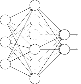
Parameter Initialization¶

If the weights are initialized in such a way that the input to each unit has a high probability of being very large (often the case when initializing to a normal distribution with high standard deviation with high fan-in), the hidden units can be heavily saturated. In this case, a small change in the input can cause almost no change in the output. As a result, a common method is to set the standard deviation to $1/\sqrt{n_{in}}$ where $n_{in}$ is the fan-in in the layer. This effectively will speed up training, and also potentially find better local minimum.

Initialization

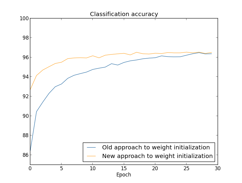
Takeaway: Weight initialization should be done with the fan-in in mind.

Momentum and NAG¶

In practice, it can be beneficial to include information about how the gradient is changing in gradient descent techniques. The ideal solution would be to compute the Hessian (second-order derivative matrix), but because its size is quadratic in the number of parameters it can be infeasible to compute and invert. A common compromise is to use momentum, which modifies the gradient descent update rule to

$\begin{align*} v &\rightarrow v^\prime = \mu v - \eta \nabla C(w)\\ w &\rightarrow w^\prime = w + v^\prime \end{align*}$ The variable

$\mu$ controls the amount that the old value of

$v$ is recycled; if it is close to

$1$ , the gradient will build up a lot of "speed"; if it's close to

$0$ the technique becomes more and more like standard gradient descent. A simple modification is Nesterov's Accelerated Gradient (NAG), which uses the update rule

$\begin{align*} v &\rightarrow v^\prime = \mu v - \eta \nabla C(w + \mu v)\\ w &\rightarrow w^\prime = w + v^\prime \end{align*}$ In effect, a partial update

$w + \mu v$ is performed to

$w$ before

$v^\prime$ is computed. This can lead to better stability in some situations. Other approximate second-order methods such as conjugate gradient and (L-)BFGS are sometimes used.

Rectified linear units (ReLUs)¶

The ReLU is an activation function/nonlinearity which simply rectifies the input:

$a = \max(0, Wx + b)$ This type of activation never saturates like sigmoidal units, but when the input is negative it has a zero gradient. They have been empirically found to work well with deep networks.

Tips for adjusting hyperparameters¶

Adjusting hyperparameters is very often done by hand, but if the initial hyperparameters used are wrong it can be hard to figure out which knob to adjust, in which direction, and by how much. Because this tuning is usually done based on validation set performance, it can be helpful to start with a simplified problem (fewer classes, less data, more frequent monitoring) which produces results more quickly. For specific hyperparameters:

Learning rate: Too large of a learning rate can cause the cost to randomly fluctuate and never settle; too small can cause it to decrease too slowly. Start by finding a small learning rate which works, then increase it until the cost starts to oscillate; set it slightly below this value. It is often helpful to decrease the learning rate once validation cost starts to plateau.
Number of epochs: Use early stopping - once the validation cost starts to increase continually, stop training.
Weight decay parameter $\lambda$ : Start without weight decay, then start small and increase until you find a value which effects the network's training dynamics.
Mini-batch size: Using larger batches can improve computational efficiency, but using smaller batches can also help to avoid local minima. Usually, it's set to be small but large enough to be efficient; around 100 training examples per minibatch. This hyperparameter is pretty independent of the others, so you can fix it first then optimize the rest.

Code Example¶

Here's a brief example which covers some of the concepts discussed above using the in-development library nntools, which provides common tools using Theano. It should replicate the model structure/hyperparameters/results from in the chapter. It's based on the mnist.py example included in nntools. Note: nntools is under active development; this code was made to work with commit ce8808f40c2949b2794f9ed4b12d7257bcc30507.

In [55]:

from __future__ import print_function

import cPickle as pickle
import gzip
import itertools
import urllib

import numpy as np
import nntools
import theano
import theano.tensor as T

# Global constants
# Filename of the MNIST pickle; get it from http://deeplearning.net/data/mnist/mnist.pkl.gz
DATA_FILENAME = 'mnist.pkl.gz'
# How many epochs must the validation loss be greater than the best so far before stopping?
NUM_BAD_EPOCHS = 100
# Size of each minibatch
BATCH_SIZE = 500
# Number of units in the single hidden layer
NUM_HIDDEN_UNITS = 100
# Learning rate (eta)
LEARNING_RATE = 0.005
# Weight decay lambda parameter
DECAY_LAMBDA = 5.

def one_hot(labels, n_classes):
    '''
    Converts an array of label integers to a one-hot matrix encoding

    :parameters:
        - labels : np.ndarray, dtype=int
            Array of integer labels, in {0, n_classes - 1}
        - n_classes : int
            Total number of classes

    :returns:
        - one_hot : np.ndarray, dtype=bool, shape=(labels.shape[0], n_classes)
            One-hot matrix of the input
    '''
    one_hot = np.zeros((labels.shape[0], n_classes)).astype(int)
    one_hot[range(labels.shape[0]), labels] = True
    return one_hot


def load_data():
    '''
    Load in the mnist.pkl data
    
    :returns:
        - dataset : dict
            A dict containing train/validation/test data/labels/shapes
    '''
    # Load in the pkl.gz
    with gzip.open(DATA_FILENAME, 'rb') as f:
        data = pickle.load(f)
    X_train, y_train = data[0]
    X_valid, y_valid = data[1]
    X_test, y_test = data[2]
    # Get the number of classes in the data (should be 10)
    num_classes = np.unique(y_train).shape[0]
    
    # Convert class numbers (ints) to one-hot representation (see above)
    y_train = one_hot(y_train, num_classes)
    y_valid = one_hot(y_valid, num_classes)
    y_test = one_hot(y_test, num_classes)

    # Construct a dataset dict
    return dict(X_train=theano.shared(nntools.utils.floatX(X_train)),
                y_train=theano.shared(nntools.utils.floatX(y_train)),
                X_valid=theano.shared(nntools.utils.floatX(X_valid)),
                y_valid=theano.shared(nntools.utils.floatX(y_valid)),
                X_test=theano.shared(nntools.utils.floatX(X_test)),
                y_test=theano.shared(nntools.utils.floatX(y_test)),
                num_examples_train=X_train.shape[0],
                num_examples_valid=X_valid.shape[0],
                num_examples_test=X_test.shape[0],
                input_dim=X_train.shape[1],
                output_dim=num_classes)


def create_iter_functions(dataset, output_layer,
                          batch_size=BATCH_SIZE,
                          learning_rate=LEARNING_RATE,
                          decay_lambda=DECAY_LAMBDA):
    '''
    Create functions for training the network and computing train/validation/test loss/accuracy
    
    :parameters:
        - dataset : dict
            Dataset dict, as returned by load_data
        - output_layer : nntools.Layer
            Output layer of a neural network you've constructed
        - batch_size : int
            Mini-batch size
        - learning_rate : float
            Learning rate for SGD optimization
        - decay_lambda : float
            Weight decay lambda hyperparameter
    
    :returns:
        - iter_funcs : dict
            Dictionary of iterator functions for training/evaluating the network
    '''
    # Mini-batch index, symbolic, for use in theano functions
    batch_index = T.iscalar('batch_index')
    # X (data) and y (output) symbolic matrices
    X_batch = T.matrix('x')
    y_batch = T.matrix('y')
    # Create a slice object for indexing X and y to obtain batches
    batch_slice = slice(batch_index * batch_size, (batch_index + 1) * batch_size)

    # Loss function for the network
    def loss(output):
        # Collect all non-bias parameters
        params = nntools.layers.get_all_non_bias_params(output_layer)
        # Loss = cross-entropy ...
        return (T.sum(-y_batch*T.log(output) - (1. - y_batch)*T.log(1. - output))
                # + weight decay
                + (decay_lambda/y_batch.shape[0])*sum(T.sum(p**2) for p in params))

    # Symbolic loss function for a batch of data
    loss_train = loss(output_layer.get_output(X_batch))
    # When using a dropout layer, we need to not drop out units when computing 
    # validation/test statistics.  We'll use this function instead
    loss_eval = loss(output_layer.get_output(X_batch, deterministic=True))

    # Compute predicted class for a batch
    pred = T.argmax(output_layer.get_output(X_batch, deterministic=True), axis=1)
    # Compute the accuracy - mean number of correct classes
    accuracy = T.mean(T.eq(pred, T.argmax(y_batch, axis=1)))

    # Collect all parameters of the network
    all_params = nntools.layers.get_all_params(output_layer)
    # Compute SGD updates for these parameters
    updates = nntools.updates.sgd(loss_train, all_params, learning_rate)

    # Create training function - includes updates
    iter_train = theano.function([batch_index], loss_train, updates=updates,
                                 givens={X_batch: dataset['X_train'][batch_slice],
                                         y_batch: dataset['y_train'][batch_slice]})

    # Create validation/test functions
    iter_valid = theano.function([batch_index], [loss_eval, accuracy],
                                 givens={X_batch: dataset['X_valid'][batch_slice],
                                         y_batch: dataset['y_valid'][batch_slice]})

    iter_test = theano.function([batch_index], [loss_eval, accuracy],
                                givens={X_batch: dataset['X_test'][batch_slice],
                                        y_batch: dataset['y_test'][batch_slice]})

    return dict(train=iter_train, valid=iter_valid, test=iter_test)


def train(iter_funcs, dataset, batch_size=BATCH_SIZE):
    '''
    Create an iterator for training using iterator functions.
    
    :parameters:
        - iter_funcs : dict
            Dictionary of iterator functions, as returned by create_iter_functions
        - dataset : dict
            Dataset dictionary, as returned by load_data
        - batch_size : int
            Mini-batch size
    
    :returns:
        - epoch_result : dict
            Statistics for each epoch, yielded after each epoch
    '''
    # Compute the number of train/validation minibatches
    num_batches_train = dataset['num_examples_train'] // batch_size
    num_batches_valid = dataset['num_examples_valid'] // batch_size

    # Count indefinitely starting from 1
    for epoch in itertools.count(1):
        # Train for one epoch over all minibatches
        batch_train_losses = []
        for b in range(num_batches_train):
            batch_train_loss = iter_funcs['train'](b)
            batch_train_losses.append(batch_train_loss)
        
        # Compute average training loss for all minibatches
        avg_train_loss = np.mean(batch_train_losses)

        # Compute validation loss/accuracy by accumulating over all batches...
        batch_valid_losses = []
        batch_valid_accuracies = []
        for b in range(num_batches_valid):
            batch_valid_loss, batch_valid_accuracy = iter_funcs['valid'](b)
            batch_valid_losses.append(batch_valid_loss)
            batch_valid_accuracies.append(batch_valid_accuracy)

        # ...and taking the mean
        avg_valid_loss = np.mean(batch_valid_losses)
        avg_valid_accuracy = np.mean(batch_valid_accuracies)

        # Yield the epoch result dict
        yield {'number': epoch,
               'train_loss': avg_train_loss,
               'valid_loss': avg_valid_loss,
               'valid_accuracy': avg_valid_accuracy}


def test_accuracy(iter_funcs, dataset, batch_size=BATCH_SIZE):
    '''
    Compute accuracy on the test set.
    
    :parameters:
        - iter_funcs : dict
            Dictionary of iterator functions, as returned by create_iter_functions
        - dataset : dict
            Dataset dictionary, as returned by load_data
        - batch_size : int
            Mini-batch size
    
    :returns:
        - test_accuracy : float
            Model accuracy on the test set
    '''
    # Compute the number of test batches
    num_batches_test = dataset['num_examples_test'] // batch_size
    # Accumulate test accuracy over all batches
    batch_accuracies = []
    for b in range(num_batches_test):
        batch_loss, batch_accuracy = iter_funcs['valid'](b)
        batch_accuracies.append(batch_accuracy)
    # Take the mean over all batches to get the actual test accuracy    
    return np.mean(batch_accuracies)

In [57]:

import IPython.display
import matplotlib.pyplot as plt
%matplotlib inline

# Load in the data dict
dataset = load_data()

# Construct the network, first with the input layer
l_in = nntools.layers.InputLayer(shape=(BATCH_SIZE, dataset['input_dim']))
# One hidden layer
l_hidden1 = nntools.layers.DenseLayer(l_in, num_units=NUM_HIDDEN_UNITS, 
                                      # Sigmoidal activation, as in the chapter
                                      nonlinearity=nntools.nonlinearities.sigmoid,
                                      # Initialize with normal with std = 1/sqrt(fan-in)
                                      W=nntools.init.Normal(std=1./np.sqrt(dataset['input_dim'])))
# Output layer
l_out = nntools.layers.DenseLayer(l_hidden1, num_units=dataset['output_dim'], 
                                  # Sigmoidal activation, as in the chapter
                                  nonlinearity=nntools.nonlinearities.sigmoid,
                                  # Initialize with normal with std = 1/sqrt(fan-in)
                                  W=nntools.init.Normal(std=1./np.sqrt(NUM_HIDDEN_UNITS)))

# Construct iterator function dictionary
iter_funcs = create_iter_functions(dataset, l_out)

# Keep track of train/validation losses for later plotting
train_losses = []
valid_losses = []
# Keep track of the best validation loss so far for early stopping
best_valid_loss = np.inf

# Try/except is so we can stop early manually
try:
    # Calling train in a for loop will train one epoch at a time
    for epoch in train(iter_funcs, dataset):
        # Print statistics of this epoch
        IPython.display.clear_output(wait=True)
        print("Epoch {}".format(epoch['number']))
        print("  training loss:\t\t{}".format(epoch['train_loss']))
        print("  validation loss:\t\t{}".format(epoch['valid_loss']))
        print("  validation accuracy:\t\t{:.3f}%".format(epoch['valid_accuracy'] * 100))
        # Store the validation/train loss for this epoch
        train_losses.append(epoch['train_loss'])
        valid_losses.append(epoch['valid_loss'])
        # If this is a new best validation loss, store it
        if epoch['valid_loss'] < best_valid_loss:
            best_valid_loss = epoch['valid_loss']
        # Otherwise, if there's not best validation loss in NUM_BAD_EPOCHS, break
        else:
            if (np.array(valid_losses)[-NUM_BAD_EPOCHS:] > best_valid_loss).all():
                break
except KeyboardInterrupt:
    pass

# Plot train/validation curves
plt.plot(train_losses, label='Train loss')
plt.plot(valid_losses, label='Validation loss')
plt.legend()

print('Test accuracy: {:.3f}%'.format(test_accuracy(iter_funcs, dataset)*100))

Epoch 511
  training loss:		136.801458913
  validation loss:		159.63904583
  validation accuracy:		98.000%
Test accuracy: 97.850%