Kalman Filters
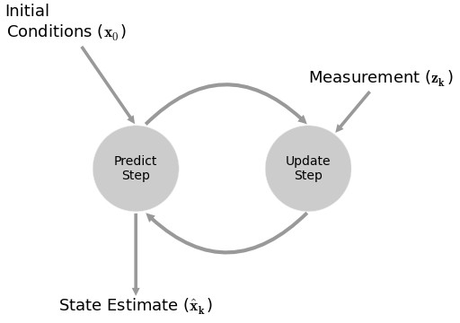
the fundamental idea is to blend somewhat inaccurate measurements with somewhat inaccurate models of how the systems behaves to get a filtered estimate that is better than either information source by itself
Pros
- filters out noise
- predictive
- adapative with future data
- does NOT require stationary data
- outputs a distribution for estimates $ (\mu, \sigma) $
- for a random walk + noise model, it can be shown to be equivalent to a EWMA (exponentially weighted moving average) [1]
- can handle missing data
- compared to other methods, found to be superior in calculating beta
Cons
- assumes linear dependencies (although there is a non-linear version)
- assumes guassian errors
- computationally is cubic to the size of the state space
Equations
$$\begin{align*} x_{t+1} &= Ax_t + Bu_t + w_t \\ z_t &= Hx_t + v_t \\ \end{align*}$$$$\begin{align*} A &= \text{predicion matrix (transition_matrices)} \\ x &= \text{states} \\ B &= \text{control matrix (transition_offsets)} \\ w &= \text{noise (transition_covariance)} \sim N(\theta, Q) \\ z &= \text{observable readings} \\ H &= \text{mapping of} \; x \; \text{to observable (observation_matrices)} \\ v &= \text{observation noise, measurement noise (observation_covariance)} \sim N(\theta, R) \end{align*}$$Best Practices
- normalize if possible
- the ratio of $ Q $ and $ R $
Calculating $ Q $
- approximate [1]
- calculate variate estimate of error in a controlled environment
- if z doesn't change, calculate variance estimate of z
- if z does change, calculate variance of regression estimate of z
- guess
- use some constant multiplied by the identity matrix
- higher the constant, higher the noise
- MLE
Example: Beta
beta_figures[0]
2015-11-05 08:15:54.476 [WARN] C:\Anaconda2\lib\site-packages\matplotlib\collections.py:590: FutureWarning: elementwise comparison failed; returning scalar instead, but in the future will perform elementwise comparison
  if self._edgecolors == str('face'):

Equations
$$ \begin{bmatrix} \beta_{t+1} \\ \alpha_{t+1} \end{bmatrix} = \begin{bmatrix} 1 & 0 \\ 0 & 1 \end{bmatrix} \begin{bmatrix} \beta_{t} \\ \alpha_{t} \end{bmatrix} + \begin{bmatrix} 0 \\ 0 \end{bmatrix} + \begin{bmatrix} w_{\beta, t} \\ w_{\alpha, t} \end{bmatrix} $$$$ r_{VIX, t} = \begin{bmatrix} r_{SPX, t} & 1 \end{bmatrix} \begin{bmatrix} \beta_{t} \\ \alpha_{t} \end{bmatrix} + v_t $$Transition Parameters
# how does beta/alpha change over time? random walk!
transition_matrices = np.eye(2)

# what is the beta/alpha drift over time? random walk!
transition_offsets = [0, 0]

# GUESS how much does beta/alpha change due to unmodeled forces?
transition_covariance = delta / (1 - delta) * np.eye(2)
Observation Parameters
# VIX returns are 1-dimensional
n_dim_obs = 1

# how do we convert beta/alpha to VIX returns
observation_matrices = np.expand_dims(
    a    = np.vstack([[x], [np.ones(len(x))]]).T,
    axis = 1
)

# GUESS how much does VIX returns deviate outside of beta/alpha estimates
observation_covariance = .01
Calculate Q and R
split into k folds
calculate MSE using pykalman's
emon previous foldskf.em( X = y_training, n_iter = 10, em_vars = ['transition_covariance', 'observation_covariance'] )use MSE in current fold

beta_figures[1]

beta_df.dropna(inplace=True)

resid_kf  = beta_df['beta'] * beta_df['x'] - beta_df['y']
resid_30  = beta_df['beta_30'] * beta_df['x'] - beta_df['y']
resid_250 = beta_df['beta_250'] * beta_df['x'] - beta_df['y']
resid_500 = beta_df['beta_500'] * beta_df['x'] - beta_df['y']

print np.sum(resid_kf**2) / len(resid_kf)
print np.sum(resid_30**2) / len(resid_30)
print np.sum(resid_250**2) / len(resid_250)
print np.sum(resid_500**2) / len(resid_500)
0.00145648345444
0.00136178536756
0.00162842090621
0.00176787087888
resid_kf  = beta_df['beta'].shift(1) * beta_df['x'] - beta_df['y']
resid_30  = beta_df['beta_30'].shift(1) * beta_df['x'] - beta_df['y']
resid_250 = beta_df['beta_250'].shift(1) * beta_df['x'] - beta_df['y']
resid_500 = beta_df['beta_500'].shift(1) * beta_df['x'] - beta_df['y']

print np.sum(resid_kf**2) / len(resid_kf)
print np.sum(resid_30**2) / len(resid_30)
print np.sum(resid_250**2) / len(resid_250)
print np.sum(resid_500**2) / len(resid_500)
0.00157659837059
0.00159214078837
0.0016753622042
0.0017999663961
beta_figures[2]

Example: Pairs Trading
$$ \begin{bmatrix} \beta_{t+1} \\ \alpha_{t+1} \end{bmatrix} = \begin{bmatrix} 1 & 0 \\ 0 & 1 \end{bmatrix} \begin{bmatrix} \beta_{t} \\ \alpha_{t} \end{bmatrix} + \begin{bmatrix} 0 \\ 0 \end{bmatrix} + \begin{bmatrix} w_{\beta, t} \\ w_{\alpha, t} \end{bmatrix} $$$$ p_{B, t} = \begin{bmatrix} p_{A, t} & 1 \end{bmatrix} \begin{bmatrix} \beta_{t} \\ \alpha_{t} \end{bmatrix} + v_t $$pairs_figures[0]

pairs_figures[1]

pairs_figures[2]

Equations
$$ \begin{align*} x_{t+1} & = f(x_t, w_t) \\ z_t & = g(x_t, v_t) \end{align*} $$f = predicion matrix (transition_functions)
x = states
w = noise ~ N(0, Q) (transition_covariance)
z = observable readings
g = mapping of x to observable (observation_functions)
v = observation noise, measurement noise ~ N(0, R) (observation_covariance)
Example: Stochastic Volatility
$$ r_t = \mu + \sqrt{\nu_t} \, w_t $$$$ \nu_{t+1} = \nu_{t} + \theta \, (\omega-\nu_t) + \xi \, \nu_t^{\kappa} \, b_t $$where $ w_t $ and $ b_t $ are correlated with a value of $ \rho $.
For Heston, $ k = 0.5 $ . For GARCH, $ k = 1.0 $. For 3/2, $ k = 1.5 $.
Let:
$$ z_t = \frac{1}{\sqrt{1 - \rho^{2}}} (b_t - \rho w_t)$$$ z_t $ and $ w_t $ are not correlated!
$$ w_t = \frac{ r_t - \mu }{ \sqrt{\nu_t} } $$$$ b_t = \sqrt{1 - \rho^{2}} \, z_t + \rho w_t $$$$ b_t = \sqrt{1 - \rho^{2}} \, z_t + \rho \frac{ r_t - \mu }{ \sqrt{\nu_t} } $$Finally...
$$ \nu_{t+1} = \nu_{t} + \theta \, (\omega-\nu_t) + \xi \, \nu_t^{\kappa} \left [ \sqrt{1 - \rho^{2}} \, z_t + \rho \frac{ r_t - \mu }{ \sqrt{\nu_t} } \right ] $$$$ r_t = \mu + \sqrt{\nu_t} w_t $$def sv_kf_functions(mu, theta, omega, xi, k, rho, log_returns):
def f(current_state, transition_noise, log_return):
b_t = math.sqrt(1 - rho ** 2) * transition_noise + rho * (r - mu) / math.sqrt(current_state)
return current_state + theta * (omega - current_state) + xi * current_state ** k * b_t
def g(current_state, observation_noise):
return mu + math.sqrt(current_state) * observation_noise
return [partial(f, log_return=log_return) for log_return in log_returns], g

About Me
I'm a trader/quant.
I started blogging on Alphamaximus
I'm also a co-founder of Bonjournal.
Follow me on Twitter.