Klasifikátory a analýza pohybu
Několik typů klasifikátorů:
- Nejbližší soused (KNN)
- Bayessův klasifikátor
- Support Vector Machine (SVM)
Dva základní typy učení:
- S učitelem (Supervised learning)
- Bez učitele (Unsupervised learning)
Klasifikátory v Pythonu
Dobrým pomocníkem je balík scikits-learn (sklearn).
%pylab inline --no-import-all
from sklearn import datasets
import numpy as np
import sklearn.model_selection
Populating the interactive namespace from numpy and matplotlib
Kosatec
Načtení trénovacích dat. Jde o kosatec (iris flower) a jeho tři poddruhy: Iris setosa, Iris versicolor, Iris virginica. Měří se délka kalichu, šířka kalichu, délka okvětního lístku a šířka okvětního lístku.

iris = datasets.load_iris()
# cílové třídy
# rozměry dat
print("data ", iris.data.shape)
print(iris.data[-10:,:])

print("")
print("target", iris.target.shape)
print(np.unique(iris.target))
print(iris.target[-10:])
('data ', (150, 4))
[[ 6.7  3.1  5.6  2.4]
 [ 6.9  3.1  5.1  2.3]
 [ 5.8  2.7  5.1  1.9]
 [ 6.8  3.2  5.9  2.3]
 [ 6.7  3.3  5.7  2.5]
 [ 6.7  3.   5.2  2.3]
 [ 6.3  2.5  5.   1.9]
 [ 6.5  3.   5.2  2. ]
 [ 6.2  3.4  5.4  2.3]
 [ 5.9  3.   5.1  1.8]]

('target', (150,))
[0 1 2]
[2 2 2 2 2 2 2 2 2 2]
Klasifikátor podle K-nejbližšího souseda
Nejbližší soused

K - nejbližší soused

Počítání minimální vzdálenosti

from sklearn import neighbors
knn = neighbors.KNeighborsClassifier()
knn.fit(iris.data, iris.target)
#KNeighborsClassifier(...)
predikce = knn.predict([[0.1, 0.2, 0.3, 0.4]])
print predikce
#array([0])
[0]

Trénovací a testovací sada
Při experimentování je důležité rozdělit data na trénovací a testovací sadu.
perm = np.random.permutation(iris.target.size)
iris.data = iris.data[perm]
iris.target = iris.target[perm]

train_data = iris.data[:100]
train_target = iris.target[:100]

test_data = iris.data[100:]
test_target = iris.target[100:]

knn.fit(train_data, train_target)

knn.score(test_data, test_target)
/usr/lib/pymodules/python2.7/sklearn/neighbors/base.py:23: UserWarning: kneighbors: neighbor k+1 and neighbor k have the same distance: results will be dependent on data order.
  warnings.warn(msg)
0.97999999999999998
Bayessův klasifikátor
import sklearn.naive_bayes
gnb = sklearn.naive_bayes.GaussianNB()
gnb.fit(train_data, train_target)
y_pred = gnb.predict(test_data)
print("Number of mislabeled points : %d" % (test_target != y_pred).sum())
Number of mislabeled points : 2
SVM klasifikátor
Rozděluje data nadrovinou

from sklearn import svm
svc = svm.SVC()
svc.fit(train_data, train_target)
y_pred = svc.predict(test_data)
print("Number of mislabeled points : %d" % (test_target != y_pred).sum())
Number of mislabeled points : 0
/usr/lib/pymodules/python2.7/sklearn/svm/classes.py:184: FutureWarning: SVM: scale_C will be True by default in scikit-learn 0.11
  cache_size, scale_C)
Učení bez učitele
Cílem je rodělit obrazy bez další informace do skupin - shluků
Vstup

výstup

Pro jednoduché případy lze použít algoritmus K-Means. Pro složitější natrénování Bayessova klasifikátoru je využíván EM-algoritmus.
Příklad klasifikace
Klasifikovat objekty v obraze

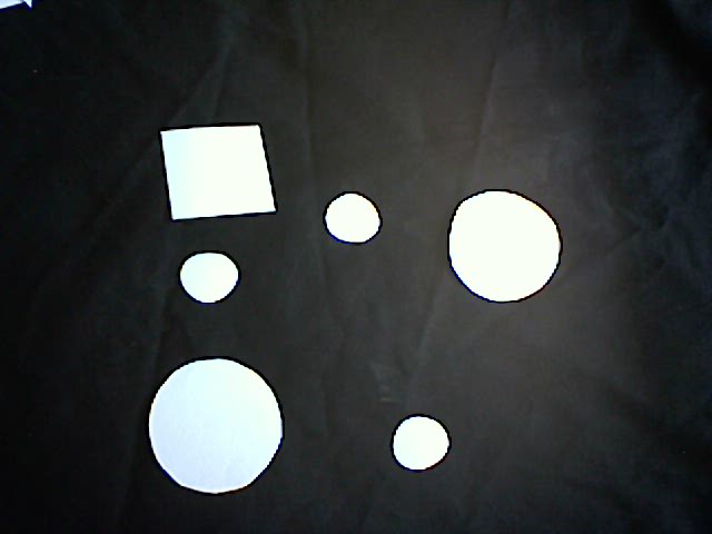
Trénovací data
https://raw.githubusercontent.com/mjirik/ZDO/master/objekty/ctverce_hvezdy_kolecka.jpg
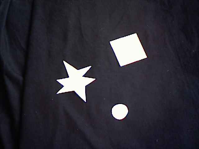
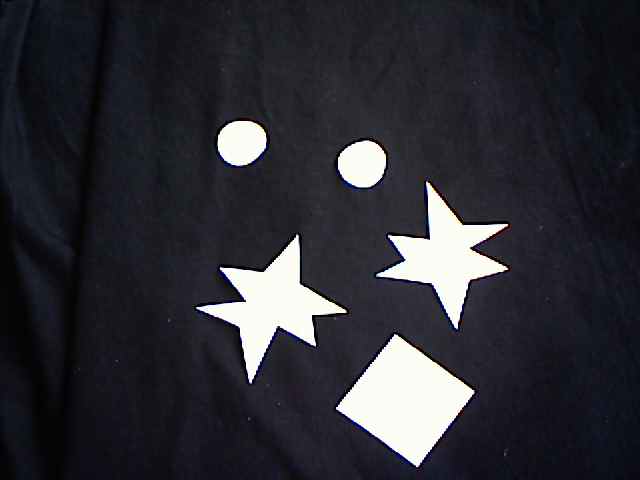
Testovací data
https://raw.githubusercontent.com/mjirik/ZDO/master/objekty/01.jpg
https://raw.githubusercontent.com/mjirik/ZDO/master/objekty/02.jpg
...
https://raw.githubusercontent.com/mjirik/ZDO/master/objekty/16.jpg
https://raw.githubusercontent.com/mjirik/ZDO/master/objekty/17.jpg
import scipy
import urllib
import cStringIO
import skimage
import skimage.color
import skimage.filter
import skimage.measure
import skimage.io
from sklearn import svm


# URL = "http://uc452cam01-kky.fav.zcu.cz/snapshot.jpg"
URL = "https://raw.githubusercontent.com/mjirik/ZDO/master/objekty/ctverce_hvezdy_kolecka.jpg"
img = skimage.io.imread(URL, as_grey=True)
plt.imshow(img)
# doporučený klasifikátor ...
# pozor na labeling a "+1 problém"
<matplotlib.image.AxesImage at 0x111887fd0>

ukázka řešení
v notes
Titanic

VARIABLE DESCRIPTIONS
- [Pclass] Passenger Class (1 = 1st; 2 = 2nd; 3 = 3rd)
- [survival] Survival (0 = No; 1 = Yes)
- name Name
- sex Sex
- age Age
- sibsp Number of Siblings/Spouses Aboard
- parch Number of Parents/Children Aboard
- ticket Ticket Number
- fare Passenger Fare (British pound)
- cabin Cabin
- embarked Port of Embarkation (C = Cherbourg; Q = Queenstown; S = Southampton)
- boat Lifeboat
- body Body Identification Number
- home.dest Home/Destination
SPECIAL NOTES
Pclass is a proxy for socio-economic status (SES) 1st ~ Upper; 2nd ~ Middle; 3rd ~ Lower
Age is in Years; Fractional if Age less than One (1) If the Age is estimated, it is in the form xx.5
Fare is in Pre-1970 British Pounds () Conversion Factors: 1 = 12s = 240d and 1s = 20d
import pandas as pd
import seaborn as sns
titanic = sns.load_dataset("titanic")
titanic
| survived | pclass | sex | age | sibsp | parch | fare | embarked | class | who | adult_male | deck | embark_town | alive | alone | |
|---|---|---|---|---|---|---|---|---|---|---|---|---|---|---|---|
| 0 | 0 | 3 | male | 22.0 | 1 | 0 | 7.2500 | S | Third | man | True | NaN | Southampton | no | False |
| 1 | 1 | 1 | female | 38.0 | 1 | 0 | 71.2833 | C | First | woman | False | C | Cherbourg | yes | False |
| 2 | 1 | 3 | female | 26.0 | 0 | 0 | 7.9250 | S | Third | woman | False | NaN | Southampton | yes | True |
| 3 | 1 | 1 | female | 35.0 | 1 | 0 | 53.1000 | S | First | woman | False | C | Southampton | yes | False |
| 4 | 0 | 3 | male | 35.0 | 0 | 0 | 8.0500 | S | Third | man | True | NaN | Southampton | no | True |
| 5 | 0 | 3 | male | NaN | 0 | 0 | 8.4583 | Q | Third | man | True | NaN | Queenstown | no | True |
| 6 | 0 | 1 | male | 54.0 | 0 | 0 | 51.8625 | S | First | man | True | E | Southampton | no | True |
| 7 | 0 | 3 | male | 2.0 | 3 | 1 | 21.0750 | S | Third | child | False | NaN | Southampton | no | False |
| 8 | 1 | 3 | female | 27.0 | 0 | 2 | 11.1333 | S | Third | woman | False | NaN | Southampton | yes | False |
| 9 | 1 | 2 | female | 14.0 | 1 | 0 | 30.0708 | C | Second | child | False | NaN | Cherbourg | yes | False |
| 10 | 1 | 3 | female | 4.0 | 1 | 1 | 16.7000 | S | Third | child | False | G | Southampton | yes | False |
| 11 | 1 | 1 | female | 58.0 | 0 | 0 | 26.5500 | S | First | woman | False | C | Southampton | yes | True |
| 12 | 0 | 3 | male | 20.0 | 0 | 0 | 8.0500 | S | Third | man | True | NaN | Southampton | no | True |
| 13 | 0 | 3 | male | 39.0 | 1 | 5 | 31.2750 | S | Third | man | True | NaN | Southampton | no | False |
| 14 | 0 | 3 | female | 14.0 | 0 | 0 | 7.8542 | S | Third | child | False | NaN | Southampton | no | True |
| 15 | 1 | 2 | female | 55.0 | 0 | 0 | 16.0000 | S | Second | woman | False | NaN | Southampton | yes | True |
| 16 | 0 | 3 | male | 2.0 | 4 | 1 | 29.1250 | Q | Third | child | False | NaN | Queenstown | no | False |
| 17 | 1 | 2 | male | NaN | 0 | 0 | 13.0000 | S | Second | man | True | NaN | Southampton | yes | True |
| 18 | 0 | 3 | female | 31.0 | 1 | 0 | 18.0000 | S | Third | woman | False | NaN | Southampton | no | False |
| 19 | 1 | 3 | female | NaN | 0 | 0 | 7.2250 | C | Third | woman | False | NaN | Cherbourg | yes | True |
| 20 | 0 | 2 | male | 35.0 | 0 | 0 | 26.0000 | S | Second | man | True | NaN | Southampton | no | True |
| 21 | 1 | 2 | male | 34.0 | 0 | 0 | 13.0000 | S | Second | man | True | D | Southampton | yes | True |
| 22 | 1 | 3 | female | 15.0 | 0 | 0 | 8.0292 | Q | Third | child | False | NaN | Queenstown | yes | True |
| 23 | 1 | 1 | male | 28.0 | 0 | 0 | 35.5000 | S | First | man | True | A | Southampton | yes | True |
| 24 | 0 | 3 | female | 8.0 | 3 | 1 | 21.0750 | S | Third | child | False | NaN | Southampton | no | False |
| 25 | 1 | 3 | female | 38.0 | 1 | 5 | 31.3875 | S | Third | woman | False | NaN | Southampton | yes | False |
| 26 | 0 | 3 | male | NaN | 0 | 0 | 7.2250 | C | Third | man | True | NaN | Cherbourg | no | True |
| 27 | 0 | 1 | male | 19.0 | 3 | 2 | 263.0000 | S | First | man | True | C | Southampton | no | False |
| 28 | 1 | 3 | female | NaN | 0 | 0 | 7.8792 | Q | Third | woman | False | NaN | Queenstown | yes | True |
| 29 | 0 | 3 | male | NaN | 0 | 0 | 7.8958 | S | Third | man | True | NaN | Southampton | no | True |
| ... | ... | ... | ... | ... | ... | ... | ... | ... | ... | ... | ... | ... | ... | ... | ... |
| 861 | 0 | 2 | male | 21.0 | 1 | 0 | 11.5000 | S | Second | man | True | NaN | Southampton | no | False |
| 862 | 1 | 1 | female | 48.0 | 0 | 0 | 25.9292 | S | First | woman | False | D | Southampton | yes | True |
| 863 | 0 | 3 | female | NaN | 8 | 2 | 69.5500 | S | Third | woman | False | NaN | Southampton | no | False |
| 864 | 0 | 2 | male | 24.0 | 0 | 0 | 13.0000 | S | Second | man | True | NaN | Southampton | no | True |
| 865 | 1 | 2 | female | 42.0 | 0 | 0 | 13.0000 | S | Second | woman | False | NaN | Southampton | yes | True |
| 866 | 1 | 2 | female | 27.0 | 1 | 0 | 13.8583 | C | Second | woman | False | NaN | Cherbourg | yes | False |
| 867 | 0 | 1 | male | 31.0 | 0 | 0 | 50.4958 | S | First | man | True | A | Southampton | no | True |
| 868 | 0 | 3 | male | NaN | 0 | 0 | 9.5000 | S | Third | man | True | NaN | Southampton | no | True |
| 869 | 1 | 3 | male | 4.0 | 1 | 1 | 11.1333 | S | Third | child | False | NaN | Southampton | yes | False |
| 870 | 0 | 3 | male | 26.0 | 0 | 0 | 7.8958 | S | Third | man | True | NaN | Southampton | no | True |
| 871 | 1 | 1 | female | 47.0 | 1 | 1 | 52.5542 | S | First | woman | False | D | Southampton | yes | False |
| 872 | 0 | 1 | male | 33.0 | 0 | 0 | 5.0000 | S | First | man | True | B | Southampton | no | True |
| 873 | 0 | 3 | male | 47.0 | 0 | 0 | 9.0000 | S | Third | man | True | NaN | Southampton | no | True |
| 874 | 1 | 2 | female | 28.0 | 1 | 0 | 24.0000 | C | Second | woman | False | NaN | Cherbourg | yes | False |
| 875 | 1 | 3 | female | 15.0 | 0 | 0 | 7.2250 | C | Third | child | False | NaN | Cherbourg | yes | True |
| 876 | 0 | 3 | male | 20.0 | 0 | 0 | 9.8458 | S | Third | man | True | NaN | Southampton | no | True |
| 877 | 0 | 3 | male | 19.0 | 0 | 0 | 7.8958 | S | Third | man | True | NaN | Southampton | no | True |
| 878 | 0 | 3 | male | NaN | 0 | 0 | 7.8958 | S | Third | man | True | NaN | Southampton | no | True |
| 879 | 1 | 1 | female | 56.0 | 0 | 1 | 83.1583 | C | First | woman | False | C | Cherbourg | yes | False |
| 880 | 1 | 2 | female | 25.0 | 0 | 1 | 26.0000 | S | Second | woman | False | NaN | Southampton | yes | False |
| 881 | 0 | 3 | male | 33.0 | 0 | 0 | 7.8958 | S | Third | man | True | NaN | Southampton | no | True |
| 882 | 0 | 3 | female | 22.0 | 0 | 0 | 10.5167 | S | Third | woman | False | NaN | Southampton | no | True |
| 883 | 0 | 2 | male | 28.0 | 0 | 0 | 10.5000 | S | Second | man | True | NaN | Southampton | no | True |
| 884 | 0 | 3 | male | 25.0 | 0 | 0 | 7.0500 | S | Third | man | True | NaN | Southampton | no | True |
| 885 | 0 | 3 | female | 39.0 | 0 | 5 | 29.1250 | Q | Third | woman | False | NaN | Queenstown | no | False |
| 886 | 0 | 2 | male | 27.0 | 0 | 0 | 13.0000 | S | Second | man | True | NaN | Southampton | no | True |
| 887 | 1 | 1 | female | 19.0 | 0 | 0 | 30.0000 | S | First | woman | False | B | Southampton | yes | True |
| 888 | 0 | 3 | female | NaN | 1 | 2 | 23.4500 | S | Third | woman | False | NaN | Southampton | no | False |
| 889 | 1 | 1 | male | 26.0 | 0 | 0 | 30.0000 | C | First | man | True | C | Cherbourg | yes | True |
| 890 | 0 | 3 | male | 32.0 | 0 | 0 | 7.7500 | Q | Third | man | True | NaN | Queenstown | no | True |
891 rows × 15 columns
Analýza obsahu
titanic["psex"] = titanic["sex"] == "male"
sns.factorplot(x="sex", kind="count", data=titanic)
<seaborn.axisgrid.FacetGrid at 0x7fe200794190>

sns.factorplot(x="class", hue="sex", kind="count", data=titanic)
<seaborn.axisgrid.FacetGrid at 0x7fe2008fa450>

g = sns.factorplot(x="class", y="survived", hue="sex", data=titanic, kind="bar")#  ,size=6 , palette="muted")
g.despine(left=True)
g.set_ylabels("survival probability")
<seaborn.axisgrid.FacetGrid at 0x7fe20081a690>

fg = sns.FacetGrid(titanic, hue="sex", aspect=3)
fg.map(sns.kdeplot, "age", shade=True)
fg.add_legend()
fg.set(xlim=(0, 80));

fg = sns.FacetGrid(titanic, hue="class", aspect=3, palette="BuPu_d")
fg.map(sns.kdeplot, "age", shade=True)
fg.set(xlim=(0, 80));
fg.add_legend()
<seaborn.axisgrid.FacetGrid at 0x7fe200488f50>

Klasifikátor
titanic_drp = titanic[["pclass", "age", "survived"]].dropna(how="any")
X = titanic_drp[["pclass", "age"]]
y = titanic_drp[["survived"]]

X_train, X_test, y_train, y_test = sklearn.model_selection.train_test_split(X, y, test_size=0.33, random_state=42)

import sklearn.naive_bayes
gnb = sklearn.naive_bayes.GaussianNB()
gnb.fit(X_train, y_train)
# #KNeighborsClassifier(...)
y_pred = gnb.predict(X_test)
y_pred
array([0, 1, 0, 1, 0, 1, 0, 0, 0, 0, 1, 0, 1, 0, 1, 0, 0, 1, 0, 1, 0, 0, 0,
       1, 0, 0, 0, 0, 0, 0, 0, 0, 1, 0, 0, 0, 0, 1, 1, 0, 0, 0, 1, 0, 1, 0,
       0, 0, 1, 1, 1, 0, 1, 0, 0, 0, 1, 0, 0, 0, 1, 0, 0, 0, 0, 1, 0, 1, 0,
       1, 0, 1, 0, 0, 0, 0, 0, 0, 0, 1, 0, 1, 0, 0, 0, 0, 0, 0, 0, 0, 1, 1,
       0, 0, 0, 0, 1, 1, 0, 0, 0, 0, 0, 0, 1, 0, 0, 1, 0, 0, 0, 0, 0, 1, 0,
       0, 0, 0, 0, 0, 1, 0, 0, 0, 1, 0, 0, 0, 0, 1, 0, 0, 0, 0, 0, 0, 0, 1,
       0, 0, 0, 0, 1, 0, 0, 0, 0, 0, 1, 0, 0, 0, 0, 0, 0, 0, 0, 0, 1, 1, 0,
       0, 0, 1, 0, 0, 1, 0, 1, 0, 1, 0, 0, 0, 1, 0, 0, 0, 0, 0, 0, 0, 1, 1,
       0, 0, 1, 1, 0, 0, 0, 0, 0, 0, 0, 1, 0, 0, 1, 0, 0, 0, 0, 0, 0, 0, 0,
       0, 0, 1, 0, 1, 0, 0, 1, 0, 1, 0, 0, 1, 1, 0, 0, 0, 0, 1, 0, 0, 0, 1,
       0, 0, 0, 0, 1, 0])
print (sklearn.metrics.classification_report(y_test, y_pred))
             precision    recall  f1-score   support

          0       0.69      0.88      0.77       137
          1       0.72      0.44      0.55        99

avg / total       0.70      0.69      0.68       236
print (sklearn.metrics.confusion_matrix(y_test, y_pred))
[[120  17]
 [ 55  44]]
včetně pohlaví
titanic_drp = titanic[["pclass", "age", "psex", "survived"]].dropna(how="any")
X = titanic_drp[["pclass", "age", "psex"]]
y = titanic_drp[["survived"]]

X_train, X_test, y_train, y_test = sklearn.model_selection.train_test_split(X, y, test_size=0.33, random_state=42)

import sklearn.naive_bayes
gnb = sklearn.naive_bayes.GaussianNB()
gnb.fit(X_train, y_train)
# #KNeighborsClassifier(...)
y_pred = gnb.predict(X_test)
print (sklearn.metrics.classification_report(y_test, y_pred))
             precision    recall  f1-score   support

          0       0.77      0.82      0.80       137
          1       0.73      0.66      0.69        99

avg / total       0.75      0.75      0.75       236
Analýza pohybu


rozdílový obraz

kumulativní obraz

Klíčové body
