Introducing the IPython Notebook
Aron Ahmadia (US Army ERDC) and David Ketcheson (KAUST)
Teaching Numerical Methods with IPython Notebooks, SciPy 2014
from IPython.core.display import HTML
css_file = './example.css'
HTML(open(css_file, "r").read())
What is an IPython Notebook?
An IPython Notebook is a:
[A] Interactive environment for writing and running code
[B] Weave of code, data, prose, equations, analysis, and visualization
[C] Tool for prototyping new code and analysis
[D] Reproducible workflow for scientific research
[E] All of the above
Writing and Running Code
The IPython Notebook consists of an ordered list of cells.
There are four important cell types:
- Code
- Markdown
- Heading
- Raw
We briefly introduce how Code Cells work here. We will return to the other three cell types later.
Code Cells
# This is a code cell made up of Python comments
# We can execute it by clicking on it with the mouse
# then clicking the "Run Cell" button
# A comment is a pretty boring piece of code
# This code cell generates "Hello, World" when executed

print "Hello, World"
Hello, World
# Code cells can also generate graphical output
%matplotlib inline
import matplotlib
matplotlib.pyplot.hist([0, 1, 2, 2, 3, 3, 3, 4, 4, 4, 10]);

Modal editor
Starting with IPython 2.0, the IPython Notebook has a modal user interface. This means that the keyboard does different things depending on which mode the Notebook is in. There are two modes: edit mode and command mode.
Edit mode
Edit mode is indicated by a green cell border and a prompt showing in the editor area:

When a cell is in edit mode, you can type into the cell, like a normal text editor.
Command mode
Command mode is indicated by a grey cell border:

When you are in command mode, you are able to edit the notebook as a whole, but not type into individual cells. Most importantly, in command mode, the keyboard is mapped to a set of shortcuts that let you perform notebook and cell actions efficiently. For example, if you are in command mode and you press c, you will copy the current cell - no modifier is needed.
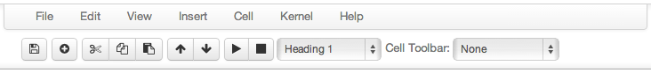
Mouse navigation
All navigation and actions in the Notebook are available using the mouse through the menubar and toolbar, which are both above the main Notebook area:
Keyboard Navigation
The modal user interface of the IPython Notebook has been optimized for efficient keyboard usage. This is made possible by having two different sets of keyboard shortcuts: one set that is active in edit mode and another in command mode.
The most important keyboard shortcuts are enter, which enters edit mode, and esc, which enters command mode.
In edit mode, most of the keyboard is dedicated to typing into the cell's editor. Thus, in edit mode there are relatively few shortcuts:
In command mode, the entire keyboard is available for shortcuts:
Here the rough order in which the IPython Developers recommend learning the command mode shortcuts:
- Basic navigation:
enter,shift-enter,up/k,down/j - Saving the notebook:
s - Cell types:
y,m,1-6,t - Cell creation and movement:
a,b,ctrl+k,ctrl+j - Cell editing:
x,c,v,d,z,shift+= - Kernel operations:
i,0
Aron and David humbly suggest learning h first!
The IPython Notebook Architecture
The centerpiece of an IPython Notebook is the "kernel", the IPython instance responsible for executing all code. Your IPython kernel maintains its state between executed cells.
x = 0
print x
0
x += 1
print x
1
Markdown cells
Text can be added to IPython Notebooks using Markdown cells. Markdown is a popular markup language that is a superset of HTML. Its specification can be found here:
Markdown basics
Text formatting
You can make text italic or bold.
Itemized Lists
- One
- Sublist
- This
- Sublist - That - The other thing
- Sublist
- Two
- Sublist
- Three
- Sublist
Enumerated Lists
- Here we go
- Sublist
- Sublist
- There we go
- Now this
Horizontal Rules
Blockquotes
To me programming is more than an important practical art. It is also a gigantic undertaking in the foundations of knowledge. -- Rear Admiral Grace Hopper
Links
Code
def f(x):
    """a docstring"""
    return x**2
You can also use triple-backticks to denote code blocks. This also allows you to choose the appropriate syntax highlighter.
if (i=0; i<n; i++) {
  printf("hello %d\n", i);
  x += 4;
}
Tables
| Time (s) | Audience Interest |
|---|---|
| 0 | High |
| 1 | Medium |
| 5 |
Images

YouTube
from IPython.display import YouTubeVideo
YouTubeVideo('vW_DRAJ0dtc')
Other HTML
Be Bold!
Mathematical Equations
Courtesy of MathJax, you can beautifully render mathematical expressions, both inline: $e^{i\pi} + 1 = 0$, and displayed:
$$e^x=\sum_{i=0}^\infty \frac{1}{i!}x^i$$Equation Environments
You can also use a number of equation environments, such as align:
A full list of available TeX and LaTeX commands is maintained by Dr. Carol Burns.
Other Useful MathJax Notes
- inline math is demarcated by
$ $, or\( \) - displayed math is demarcated by
$$ $$or\[ \] - displayed math environments can also be directly demarcated by
\beginand\end \newcommandand\defare supported, within areas MathJax processes (such as in a\[ \]block)- equation numbering is not officially supported, but it can be indirectly enabled
A Note about Notebook Security
By default, a notebook downloaded to a new computer is untrusted
- HTML and Javascript in Markdown cells is now never executed
- HTML and Javascript code outputs must be explicitly re-executed
- Some of these restrictions can be mitigrated through shared accounts (Sage MathCloud) and secrets
Magics
IPython kernels execute a superset of the Python language. The extension functions, commonly referred to as magics, come in two variants.
Line Magics
- A line magic looks like a command line call. The most important of these is
%matplotlib inline, which embeds all matplotlib plot output as images in the notebook itself.
%matplotlib inline
%whos
Variable       Type      Data/Info
----------------------------------
YouTubeVideo   type      <class 'IPython.lib.display.YouTubeVideo'>
matplotlib     module    <module 'matplotlib' from<...>matplotlib/__init__.pyc'>
x              int       1
Cell Magics
- A cell magic takes its entire cell as an argument. Although there are a number of useful cell magics, you may find
%%timeitto be useful for exploring code performance.
%%timeit

import numpy as np
np.sum(np.random.rand(1000))
10000 loops, best of 3: 23.2 µs per loop
Interacting with the Command Line
IPython supports one final trick, the ability to interact directly with your shell by using the ! operator.
!ls
Aliasing.ipynb                         Markdown Cells.ipynb                   README.md                              finite_difference_lab.ipynb
Introducing the IPython Notebook.ipynb Multigrid.ipynb                        example.css                            images
x = !ls
print x
['Aliasing.ipynb', 'Introducing the IPython Notebook.ipynb', 'Markdown Cells.ipynb', 'Multigrid.ipynb', 'README.md', 'example.css', 'finite_difference_lab.ipynb', 'images']
A Note about Notebook Version Control
The IPython Notebook is stored using canonicalized JSON for ease of use with version control systems.
There are two things to be aware of:
By default, IPython embeds all content and saves kernel execution numbers. You may want to get in the habit of clearing all cells before committing.
As of IPython 2.0, all notebooks are signed on save. This increases the chances of a commit collision during merge, forcing a manual resolution. Either signature can be safely deleted in this situation.