Scalar and vector
Marcos Duarte, Renato Naville Watanabe
Laboratory of Biomechanics and Motor Control
Federal University of ABC, Brazil
Python handles very well all mathematical operations with numeric scalars and vectors and you can use Sympy for similar stuff but with abstract symbols. Let's briefly review scalars and vectors and show how to use Python for numerical calculation.
For a review about scalars and vectors, see chapter 2 of Ruina and Rudra's book.
Python setup
from IPython.display import IFrame
import math
import numpy as np
a = 2
b = 3
print('a =', a, ', b =', b)
print('a + b =', a + b)
print('a - b =', a - b)
print('a * b =', a * b)
print('a / b =', a / b)
print('a ** b =', a ** b)
print('sqrt(b) =', math.sqrt(b))
a = 2 , b = 3
a + b = 5
a - b = -1
a * b = 6
a / b = 0.6666666666666666
a ** b = 8
sqrt(b) = 1.7320508075688772
If you have a set of numbers, or an array, it is probably better to use Numpy; it will be faster for large data sets, and combined with Scipy, has many more mathematical funcions.
a = 2
b = [3, 4, 5, 6, 7, 8]
b = np.array(b)
print('a =', a, ', b =', b)
print('a + b =', a + b)
print('a - b =', a - b)
print('a * b =', a * b)
print('a / b =', a / b)
print('a ** b =', a ** b)
print('np.sqrt(b) =', np.sqrt(b))  # use numpy functions for numpy arrays
a = 2 , b = [3 4 5 6 7 8]
a + b = [ 5  6  7  8  9 10]
a - b = [-1 -2 -3 -4 -5 -6]
a * b = [ 6  8 10 12 14 16]
a / b = [0.66666667 0.5        0.4        0.33333333 0.28571429 0.25      ]
a ** b = [  8  16  32  64 128 256]
np.sqrt(b) = [1.73205081 2.         2.23606798 2.44948974 2.64575131 2.82842712]
Numpy performs the arithmetic operations of the single number in a with all the numbers of the array b. This is called broadcasting in computer science.
Even if you have two arrays (but they must have the same size), Numpy handles for you:
a = np.array([1, 2, 3])
b = np.array([4, 5, 6])
print('a =', a, ', b =', b)
print('a + b =', a + b)
print('a - b =', a - b)
print('a * b =', a * b)
print('a / b =', a / b)
print('a ** b =', a ** b)
a = [1 2 3] , b = [4 5 6]
a + b = [5 7 9]
a - b = [-3 -3 -3]
a * b = [ 4 10 18]
a / b = [0.25 0.4  0.5 ]
a ** b = [  1  32 729]
Vector
A vector is a quantity with magnitude (or length) and direction expressed numerically as an ordered list of values according to a coordinate reference system.
For example, position, force, and torque are physical quantities defined by vectors.
For instance, consider the position of a point in space represented by a vector:
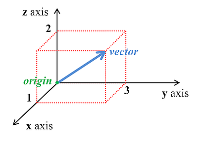
The position of the point (the vector) above can be represented as a tuple of values:
$$ (x,\: y,\: z) \; \Rightarrow \; (1, 3, 2) $$or in matrix form:
$$ \begin{bmatrix} x \\y \\z \end{bmatrix} \;\; \Rightarrow \;\; \begin{bmatrix} 1 \\3 \\2 \end{bmatrix}$$We can use the Numpy array to represent the components of vectors.
For instance, for the vector above is expressed in Python as:
a = np.array([1, 3, 2])
print('a =', a)
a = [1 3 2]
Exactly like the arrays in the last example for scalars, so all operations we performed will result in the same values, of course.
However, as we are now dealing with vectors, now some of the operations don't make sense. For example, for vectors there are no multiplication, division, power, and square root in the way we calculated.
A vector can also be represented as:
$$ \overrightarrow{\mathbf{a}} = a_x\hat{\mathbf{i}} + a_y\hat{\mathbf{j}} + a_z\hat{\mathbf{k}} $$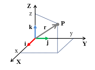
Where $\hat{\mathbf{i}},\, \hat{\mathbf{j}},\, \hat{\mathbf{k}}\,$ are unit vectors, each representing a direction and $ a_x\hat{\mathbf{i}},\: a_y\hat{\mathbf{j}},\: a_z\hat{\mathbf{k}} $ are the vector components of the vector $\overrightarrow{\mathbf{a}}$.
A unit vector (or versor) is a vector whose length (or norm) is 1.
The unit vector of a non-zero vector $\overrightarrow{\mathbf{a}}$ is the unit vector codirectional with $\overrightarrow{\mathbf{a}}$:
Magnitude (length or norm) of a vector
The magnitude (length) of a vector is often represented by the symbol $||\;||$, also known as the norm (or Euclidean norm) of a vector and it is defined as:
$$ ||\overrightarrow{\mathbf{a}}|| = \sqrt{a_x^2+a_y^2+a_z^2} $$ The function `numpy.linalg.norm` calculates the norm:a = np.array([1, 2, 3])
np.linalg.norm(a)
3.7416573867739413
Or we can use the definition and compute directly:
np.sqrt(np.sum(a*a))
3.7416573867739413
Then, the versor for the vector $ \overrightarrow{\mathbf{a}} = (1, 2, 3) $ is:
a = np.array([1, 2, 3])
u = a/np.linalg.norm(a)
print('u =', u)
u = [0.26726124 0.53452248 0.80178373]
And we can verify its magnitude is indeed 1:
np.linalg.norm(u)
1.0
Vecton addition and subtraction
The addition of two vectors is another vector:
$$ \overrightarrow{\mathbf{a}} + \overrightarrow{\mathbf{b}} = (a_x\hat{\mathbf{i}} + a_y\hat{\mathbf{j}} + a_z\hat{\mathbf{k}}) + (b_x\hat{\mathbf{i}} + b_y\hat{\mathbf{j}} + b_z\hat{\mathbf{k}}) = (a_x+b_x)\hat{\mathbf{i}} + (a_y+b_y)\hat{\mathbf{j}} + (a_z+b_z)\hat{\mathbf{k}} $$
The subtraction of two vectors is also another vector:
$$ \overrightarrow{\mathbf{a}} - \overrightarrow{\mathbf{b}} = (a_x\hat{\mathbf{i}} + a_y\hat{\mathbf{j}} + a_z\hat{\mathbf{k}}) + (b_x\hat{\mathbf{i}} + b_y\hat{\mathbf{j}} + b_z\hat{\mathbf{k}}) = (a_x-b_x)\hat{\mathbf{i}} + (a_y-b_y)\hat{\mathbf{j}} + (a_z-b_z)\hat{\mathbf{k}} $$
Consider two 2D arrays (rows and columns) representing the position of two objects moving in space. The columns represent the vector components and the rows the values of the position vector in different instants.
Once again, it's easy to perform addition and subtraction with these vectors:
a = np.array([[1, 2, 3], [1, 1, 1]])
b = np.array([[4, 5, 6], [7, 8, 9]])
print('a =', a, '\nb =', b)
print('a + b =', a + b)
print('a - b =', a - b)
a = [[1 2 3]
 [1 1 1]]
b = [[4 5 6]
 [7 8 9]]
a + b = [[ 5  7  9]
 [ 8  9 10]]
a - b = [[-3 -3 -3]
 [-6 -7 -8]]
Numpy can handle a N-dimensional array with the size limited by the available memory in your computer.
And we can perform operations on each vector, for example, calculate the norm of each one.
First let's check the shape of the variable a using the method shape or the function numpy.shape:
print(a.shape)
print(np.shape(a))
(2, 3)
(2, 3)
This means the variable a has 2 rows and 3 columns.
We have to tell the function numpy.norm to calculate the norm for each vector, i.e., to operate through the columns of the variable a using the paraneter axis:
np.linalg.norm(a, axis=1)
array([3.74165739, 1.73205081])
Dot product
Dot product (or scalar product or inner product) between two vectors is a mathematical operation algebraically defined as the sum of the products of the corresponding components (maginitudes in each direction) of the two vectors. The result of the dot product is a single number (a scalar).
The dot product between vectors $\overrightarrow{\mathbf{a}}$ and $\overrightarrow{\mathbf{b}}$ is:
Because by definition:
$$ \hat{\mathbf{i}} \cdot \hat{\mathbf{i}} = \hat{\mathbf{j}} \cdot \hat{\mathbf{j}} = \hat{\mathbf{k}} \cdot \hat{\mathbf{k}}= 1 \quad \text{and} \quad \hat{\mathbf{i}} \cdot \hat{\mathbf{j}} = \hat{\mathbf{i}} \cdot \hat{\mathbf{k}} = \hat{\mathbf{j}} \cdot \hat{\mathbf{k}} = 0 $$The geometric equivalent of the dot product is the product of the magnitudes of the two vectors and the cosine of the angle between them:
$$ \overrightarrow{\mathbf{a}} \cdot \overrightarrow{\mathbf{b}} = ||\overrightarrow{\mathbf{a}}||\:||\overrightarrow{\mathbf{b}}||\:cos(\theta) $$Which is also equivalent to state that the dot product between two vectors $\overrightarrow{\mathbf{a}}$ and $\overrightarrow{\mathbf{b}}$ is the magnitude of $\overrightarrow{\mathbf{a}}$ times the magnitude of the component of $\overrightarrow{\mathbf{b}}$ parallel to $\overrightarrow{\mathbf{a}}$ (or the magnitude of $\overrightarrow{\mathbf{b}}$ times the magnitude of the component of $\overrightarrow{\mathbf{a}}$ parallel to $\overrightarrow{\mathbf{b}}$).
The Numpy function for the dot product is numpy.dot:
a = np.array([1, 2, 3])
b = np.array([4, 5, 6])
print('a =', a, '\nb =', b)
print('np.dot(a, b) =', np.dot(a, b))
a = [1 2 3]
b = [4 5 6]
np.dot(a, b) = 32
Or we can use the definition and compute directly:
np.sum(a*b)
32
For 2D arrays, the numpy.dot function performs matrix multiplication rather than the dot product; so let's use the numpy.sum function:
a = np.array([[1, 2, 3], [1, 1, 1]])
b = np.array([[4, 5, 6], [7, 8, 9]])
np.sum(a*b, axis=1)
array([32, 24])
Vector product
Cross product or vector product between two vectors is a mathematical operation in three-dimensional space which results in a vector perpendicular to both of the vectors being multiplied and a length (norm) equal to the product of the perpendicular components of the vectors being multiplied (which is equal to the area of the parallelogram that the vectors span).
The cross product between vectors $\overrightarrow{\mathbf{a}}$ and $\overrightarrow{\mathbf{b}}$ is:
Because by definition:
$$ \begin{array}{l l} \hat{\mathbf{i}} \times \hat{\mathbf{i}} = \hat{\mathbf{j}} \times \hat{\mathbf{j}} = \hat{\mathbf{k}} \times \hat{\mathbf{k}} = 0 \\ \hat{\mathbf{i}} \times \hat{\mathbf{j}} = \hat{\mathbf{k}}, \quad \hat{\mathbf{k}} \times \hat{\mathbf{k}} = \hat{\mathbf{i}}, \quad \hat{\mathbf{k}} \times \hat{\mathbf{i}} = \hat{\mathbf{j}} \\ \hat{\mathbf{j}} \times \hat{\mathbf{i}} = -\hat{\mathbf{k}}, \quad \hat{\mathbf{k}} \times \hat{\mathbf{j}}= -\hat{\mathbf{i}}, \quad \hat{\mathbf{i}} \times \hat{\mathbf{k}} = -\hat{\mathbf{j}} \end{array} $$The direction of the vector resulting from the cross product between the vectors $\overrightarrow{\mathbf{a}}$ and $\overrightarrow{\mathbf{b}}$ is given by the right-hand rule.
The geometric equivalent of the cross product is:
The geometric equivalent of the cross product is the product of the magnitudes of the two vectors and the sine of the angle between them:
$$ \overrightarrow{\mathbf{a}} \times \overrightarrow{\mathbf{b}} = ||\overrightarrow{\mathbf{a}}||\:||\overrightarrow{\mathbf{b}}||\:sin(\theta) $$Which is also equivalent to state that the cross product between two vectors $\overrightarrow{\mathbf{a}}$ and $\overrightarrow{\mathbf{b}}$ is the magnitude of $\overrightarrow{\mathbf{a}}$ times the magnitude of the component of $\overrightarrow{\mathbf{b}}$ perpendicular to $\overrightarrow{\mathbf{a}}$ (or the magnitude of $\overrightarrow{\mathbf{b}}$ times the magnitude of the component of $\overrightarrow{\mathbf{a}}$ perpendicular to $\overrightarrow{\mathbf{b}}$).
The definition above, also implies that the magnitude of the cross product is the area of the parallelogram spanned by the two vectors:

The cross product can also be calculated as the determinant of a matrix:
$$ \overrightarrow{\mathbf{a}} \times \overrightarrow{\mathbf{b}} = \left| \begin{array}{ccc} \hat{\mathbf{i}} & \hat{\mathbf{j}} & \hat{\mathbf{k}} \\ a_x & a_y & a_z \\ b_x & b_y & b_z \end{array} \right| = a_y b_z \hat{\mathbf{i}} + a_z b_x \hat{\mathbf{j}} + a_x b_y \hat{\mathbf{k}} - a_y b_x \hat{\mathbf{k}}-a_z b_y \hat{\mathbf{i}} - a_x b_z \hat{\mathbf{j}} \\ \overrightarrow{\mathbf{a}} \times \overrightarrow{\mathbf{b}} = (a_yb_z-a_zb_y)\hat{\mathbf{i}} + (a_zb_x-a_xb_z)\hat{\mathbf{j}} + (a_xb_y-a_yb_x)\hat{\mathbf{k}} $$The same result as before.
The Numpy function for the cross product is numpy.cross:
print('a =', a, '\nb =', b)
print('np.cross(a, b) =', np.cross(a, b))
a = [[1 2 3]
 [1 1 1]]
b = [[4 5 6]
 [7 8 9]]
np.cross(a, b) = [[-3  6 -3]
 [ 1 -2  1]]
For 2D arrays with vectors in different rows:
a = np.array([[1, 2, 3], [1, 1, 1]])
b = np.array([[4, 5, 6], [7, 8, 9]])
np.cross(a, b, axis=1)
array([[-3,  6, -3],
       [ 1, -2,  1]])
Further reading
- Read pages 44-92 of the first chapter of the Ruina and Rudra's book about scalars and vectors in Mechanics.
Video lectures on the Internet
- Khan Academy: Vectors
- Vectors, what even are they?
Problems
Given the vectors, $\overrightarrow{\mathbf{a}}=[1, 0, 0]$ and $\overrightarrow{\mathbf{b}}=[1, 1, 1]$, calculate the dot and cross products between them.
Calculate the unit vectors for $[2, −2, 3]$ and $[3, −3, 2]$ and determine an orthogonal vector to these two vectors.
Given the vectors $\overrightarrow{\mathbf{a}}$=[1, 0, 0] and $\overrightarrow{\mathbf{b}}$=[1, 1, 1], calculate $ \overrightarrow{\mathbf{a}} \times \overrightarrow{\mathbf{b}} $ and verify that this vector is orthogonal to vectors $\overrightarrow{\mathbf{a}}$ and $\overrightarrow{\mathbf{b}}$. Also, calculate $\overrightarrow{\mathbf{b}} \times \overrightarrow{\mathbf{a}}$ and compare it with $\overrightarrow{\mathbf{a}} \times \overrightarrow{\mathbf{b}}$.
Given the vectors $[1, 1, 0]; [1, 0, 1]; [0, 1, 1]$, calculate a basis using the Gram–Schmidt process.
Write a Python function to calculate a basis using the Gram–Schmidt process (implement the algorithm!) considering that the input are three variables where each one contains the coordinates of vectors as columns and different positions of these vectors as rows. For example, sample variables can be generated with the command
np.random.randn(5, 3).Study the sample problems 1.1 to 1.9, 1.11 (using Python), 1.12, 1.14, 1.17, 1.18 to 1.24 of Ruina and Rudra's book
From Ruina and Rudra's book, solve the problems 1.1.1 to 1.3.16.
If you are new to scalars and vectors, you should solve these problems first by hand and then use Python to check the answers.
References
- Ruina A, Rudra P (2019) Introduction to Statics and Dynamics. Oxford University Press.