Python para análisis de datos
![]()
Juan Luis Cano Rodríguez < juanlu001@gmail.com >
Data Science Spain, Madrid 2014-07-15
Índice
- Introducción
- Bibliotecas: numpy, matplotlib, pandas
- IPython y su filosofía
- Instalación: Anaconda
- Python en España
¿Quién soy yo?
- Casi ingeniero aeronáutico por la UPM
- Fortran
7790,Excel, MATLAB y Python - Pybonacci: blog sobre Python científico en español http://pybonacci.wordpress.com/
- Presidente de la Asociación Python España http://www.es.python.org/
- Becario en Airbus
¿Qué es Python?
- Lenguaje de propósito general dinámico y fácil de aprender*
- Desarrollado por voluntarios, libre (estilo BSD) y mantenido por una fundación (PSF)
- Usos: lenguaje de scripting, servidores web, computación científica...
- A partir de ~2010, análisis de datos
* "Python es ya el lenguaje de introducción más popular en las universidades norteamericanas" http://www.genbetadev.com/formacion/python-es-ya-el-lenguaje-de-introduccion-mas-popular-en-las-universidades-norteamericanas
In [1]:
print("Hello, world!")
Hello, world!
In [2]:
def fib(N):
    a, b = 0, 1
    for ii in range(N):
        a, b = b, a + b
    return b

for ii in range(8):
    print(fib(ii))
1
1
2
3
5
8
13
21
Lenguaje de propósito general
- Sintaxis cuidadosamente diseñada
- Interfaz con multitud de bibliotecas diferentes
- Mayor variedad de herramientas de desarrollo
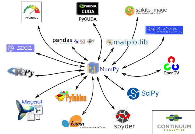
NumPy
- NumPy es el pilar fundamental de todo el ecosistema numérico en Python http://www.numpy.org/
- Arrays N-dimensionales: almacenamiento en memoria eficiente
- Funciones para operar eficientemente con ellos: operaciones vectorizadas
- Además: álgebra lineal, FFTs, números aleatorios, funciones financieras
Motivación:
"Make [Python] equivalent to a basic scientific calculator."
In [3]:
import numpy as np
In [4]:
np.array([
    [1, 2, 3],
    [4, 5, 6]
])
Out[4]:
array([[1, 2, 3],
       [4, 5, 6]])
In [5]:
np.linspace(0, 10, 5)
Out[5]:
array([ 0. , 2.5, 5. , 7.5, 10. ])
In [6]:
_.mean()
Out[6]:
5.0
Desventajas
- Pensado para conjuntos de datos de tamaño fijo
- No optimizado para datos heterogéneos (números, texto, fechas)
- Manejo de datos textuales engorroso
Solución: pandas
pandas
- Estructura de datos de alto nivel y optimizada para análisis de datos: DataFrame http://pandas.pydata.org/
- Herramientas para leer y escribir datos en diversos formatos: CSV y texto, Excel, bases de datos SQL, HDF5
- Manejo de series temporales
- Tamaño flexible, merge y join de varios DataFrames...
- Tutorial en español: http://pybonacci.wordpress.com/2014/05/30/pandas-i/
In [7]:
import pandas as pd
In [8]:
pd.Series([1, 3, 5, np.nan, 6, 8])
Out[8]:
0     1
1     3
2     5
3   NaN
4     6
5     8
dtype: float64
In [9]:
dates = pd.date_range('20140701', periods=6)
dates
Out[9]:
<class 'pandas.tseries.index.DatetimeIndex'>
[2014-07-01, ..., 2014-07-06]
Length: 6, Freq: D, Timezone: None
In [10]:
datos = pd.DataFrame(np.random.randn(6,4), index=dates,
                     columns=list('ABCD'))
datos
Out[10]:
| A | B | C | D | |
|---|---|---|---|---|
| 2014-07-01 | -0.278300 | 0.424450 | -1.508621 | -1.746290 |
| 2014-07-02 | 0.941110 | 0.050437 | 0.371443 | -0.508548 |
| 2014-07-03 | 0.761886 | 1.308292 | 0.871853 | 0.548142 |
| 2014-07-04 | 1.972977 | 0.213835 | -1.778572 | -0.165594 |
| 2014-07-05 | -0.783794 | -1.057578 | 0.067174 | -0.141001 |
| 2014-07-06 | 0.326622 | -1.085902 | -0.236260 | -0.403086 |
6 rows × 4 columns
In [11]:
datos.describe()
Out[11]:
| A | B | C | D | |
|---|---|---|---|---|
| count | 6.000000 | 6.000000 | 6.000000 | 6.000000 |
| mean | 0.490083 | -0.024411 | -0.368831 | -0.402730 |
| std | 0.971202 | 0.920232 | 1.056548 | 0.754353 |
| min | -0.783794 | -1.085902 | -1.778572 | -1.746290 |
| 25% | -0.127069 | -0.780575 | -1.190531 | -0.482183 |
| 50% | 0.544254 | 0.132136 | -0.084543 | -0.284340 |
| 75% | 0.896304 | 0.371796 | 0.295376 | -0.147149 |
| max | 1.972977 | 1.308292 | 0.871853 | 0.548142 |
8 rows × 4 columns
matplotlib
- El estándar de visualización 2D en Python http://matplotlib.org/
- Inspirada en MATLAB
- Aprendizaje costoso, pero extremadamente versátil
In [12]:
import matplotlib.pyplot as plt
%matplotlib inline
In [13]:
datos["A"].plot()
Out[13]:
<matplotlib.axes.AxesSubplot at 0x7fd6a471ed10>

In [14]:
datos["A"].plot()
plt.xlabel("Fecha")
plt.ylabel("Columna A")
plt.legend(["Datos"])
plt.title("Gráfica 1")
Out[14]:
<matplotlib.text.Text at 0x7fd6a4189090>

Otras bibliotecas
- Computación científica general: SciPy http://www.scipy.org/
- ggplot2 en Python: ggplot http://ggplot.yhathq.com/
- Aprendizaje automático (machine learning): scikit-learn http://scikit-learn.org
- Modelos y tests estadísticos: StatsModels http://statsmodels.sourceforge.net/
- Manejo de volúmenes grandes de datos: PyTables http://www.pytables.org/
¡Y mucho más!
IPython y el notebook
- IPython es un intérprete de Python mejorado http://ipython.org/
- Inspirado en el notebook de Mathematica
- Ayuda en línea, autocompletado, mejoras en la depuración...
La joya de la corona: el notebook
- Documento interactivo dividido en celdas
- Mezcla de código con texto, HTML, vídeo, imágenes...
- Gráficos incrustados, animaciones...
- Formato fácil de exportar y compartir: http://nbviewer.ipython.org/
¿Por qué usar solo Python?
In [16]:
X = np.array([0,1,2,3,4])
Y = np.array([3,5,4,6,7])
In [17]:
%load_ext rpy2.ipython
In [18]:
%Rpush X Y
%R lm(Y~X)$coef
Out[18]:
<FloatVector - Python:0x7fd6a2fdf5f0 / R:0x2d86ec8>
[3.200000, 0.900000]
In [19]:
b = %R a=resid(lm(Y~X))
%Rpull a
print(a)
%R -o a
   1    2    3    4    5
-0.2  0.9 -1.0  0.1  0.2
In [20]:
%%R -i X,Y -o XYcoef
XYlm = lm(Y~X)
XYcoef = coef(XYlm)
print(summary(XYlm))
par(mfrow=c(2,2))
plot(XYlm)
Call:
lm(formula = Y ~ X)

Residuals:
   1    2    3    4    5
-0.2  0.9 -1.0  0.1  0.2

Coefficients:
            Estimate Std. Error t value Pr(>|t|)
(Intercept)   3.2000     0.6164   5.191   0.0139 *
X             0.9000     0.2517   3.576   0.0374 *
---
Signif. codes:  0 ‘***’ 0.001 ‘**’ 0.01 ‘*’ 0.05 ‘.’ 0.1 ‘ ’ 1

Residual standard error: 0.7958 on 3 degrees of freedom
Multiple R-squared:   0.81,	Adjusted R-squared:  0.7467
F-statistic: 12.79 on 1 and 3 DF,  p-value: 0.03739

Puedo usar esta técnica con multitud de lenguajes:
- MATLAB https://github.com/arokem/python-matlab-bridge
- Octave http://blink1073.github.io/oct2py/docs/
- ¡Fortran! http://nbviewer.ipython.org/github/mgaitan/fortran_magic/blob/master/documentation.ipynb
¡y más! https://github.com/ipython/ipython/wiki/Extensions-Index
P: ¿Por qué lo llaman IPython si puede iteractuar con multitud de lenguajes diferentes?
Distribuciones de Python: Anaconda
- En Windows especialmente, instalar individualmente cada una de las bibliotecas es una pesadilla
- Incluso en Linux o OS X el problema se complica si necesitamos versiones diferentes
- Solución: distribuciones monolíticas
- Anaconda, de Continuum Analytics https://store.continuum.io/cshop/anaconda
- Otras: Pyzo, WinPython, Canopy, Python(x,y)...
La comunidad Python española
- Python Madrid http://www.meetup.com/Madrid-Python-Meetup/
- Asociación Python España http://www.es.python.org/
- Calendario de eventos y meetups nacionales http://calendario.es.python.org/
- ¡Hazte socio! http://www.es.python.org/page/quiero-ser-socio
- Primera conferencia nacional: PyCon España 2013 http://2013.es.pycon.org/
- ¡Estamos preparando la segunda en Zaragoza! http://2014.es.pycon.org/
**Muchas gracias :)**