#!/usr/bin/env python
# coding: utf-8
# # Local Search in Discrete State and Action Spaces
#
# For some search problems, the path to reach the goal is not
# important. Discovering a goal state or a state with the best value of
# some objective function is the important part. Such problems are
# often called **optimization problems**.
#
# What are some examples?
#
# What is the best setting for a control on your stove to cook your soup
# as quickly as possible without burning it?
#
# What is the best way to pack the words of a word cloud, or a [wordle](http://www.wordle.net)? See an answer [here](https://stackoverflow.com/questions/342687/algorithm-to-implement-a-word-cloud-like-wordle).
#
# What is the best way to divide up the computations of a matrix
# calculation to be distributed across multiple cores?
# **Local search** algorithms operate by maintaining a single state (or
# set of pretty good states) and generating another state to try based
# on this limited memory. Some set of actions are available to modify a
# state to another "neighboring" state. It is a "neighbor" state in an
# abstract graph of states connected by single actions.
#
# Imagine all of the possible states for a problem laid out along a
# line, along an x-axis. The value of the objective function can be
# plotted as a height above the points on the x-axis. A local search
# algorithm tries to find the state with the best height, where best
# could be the maximal or minimal value depending on the search
# problem. The best value over all states is the **global optimum** (a
# minimum or a maximum depending on the problem).
#
# A local search algorithm is **complete** if it always finds a goal
# state. It is **optimal** if it always finds the optimum state, the
# one with the global maximum or minimum.
# # Hill-Climbing Search
# This is our first example of a local search algorithm. Imagine you
# are climbing a mountain and you are in a very thick fog. You can only
# see a distance equal to one step length. To try to climb you take the
# step in the direction that is steepest to get to the highest
# point of all the locations you can currently see.
#
# In other words, hill-climbing search simply evaluates the objective
# function for all states that are neighbors to the current state, and
# takes the neighbor state with the best objective function value as the
# new current state. If there are more than one next best states, one
# is picked randomly.
#
# Hill-climbing search is sometimes called **greedy search**, because a
# step is taken after only considering the immediate neighbors. No time
# is spent considering possible future states.
#
# Hill-climbing is easy to formulate and implement and often finds
# pretty good states quickly. But, it has the following problems:
#
# * it gets stuck on local optima (hills for maximizing searches, valleys for minimizing searches,
# * it may get stuck on a ridge, if no single action can advance the search along the ridge,
# * it may get stuck wandering on a plateau for which all neighboring states have equal value.
#
# Common variations include
# * allow sideways moves (when on a plateau)
# * stochastic hill-climbing: choose next state with probability related to increase in value of objective function
# * first-choice hill-climbing: generate neighbors by random choice of available actions and keep first state that has better value,
# * random-restart hill climbing: conduct multiple hill-climbing searches from multiple, randomly generated, initial states.
#
# Only this last one, with random-restarts, is **complete**. In the limit, all states will be tried as starting states so the goal, or best state, will eventually be found.
# # The Eight-Queens Problem
# Place eight queens on a chess board so that no queen is attacking
# another. Each queen must be in one of the 8 columns, so each queen
# can be placed in one of the 8 rows, for a total of $8^8 \approx 17$
# million states. Actions are moving a single queen to a different row
# in the same column. The objective function is the number of pairs of
# queens attacking each other. This function is to be minimized, of
# course. See [this animation](https://www.youtube.com/watch?v=ckC2hFdLff0)
# and [this nice explanation](https://www.youtube.com/watch?v=jPcBU0Z2Hj8)
#
# Hill-climbing search as described only finds solutions 14% of the time, but solves those instances quickly, in an average of 4 steps. When it gets stuck this is discovered in an average of 3 steps.
#
# | Hill-climbing Variations | Percent Solved | Steps to Find Solution | Steps to Know Failure |
# | :--: |:--: |:--: |:--: |
# | basic | 14% | 4 | 3 |
# | with sideways moves | 94% | 21 | 64 |
# | with restarts | 100% | 22 | |
# | with sidways moves and restarts | 100% | 28 | |
# # Hard Problems
#
# Hard ones for hill-climbing are ones with many local optima. NP-hard problems often have an exponential number of local optima, but states with pretty good value can often be found with a small number of restarts.
# # Simulated Annealing
#
# Hill-climbing searches will get stuck on local optima. Only by adding
# random restarts can you have a hill-climbing algorithm that is
# complete.
#
# To get off of a local optimum, a search must be defined to allow steps
# that are "downhill" for maximizing searches, and "uphill" for
# minimizing searches, away from the optimum.
#
# **Simulated annealing**
# is an algorithm that does this probabilisitically. Assume we are
# doing a maximizing search, meaning we want to find the state with the
# maximum value. Let the value of
# the current state be $v$. Imagine an action has been applied to that
# state and the resulting state has a lower (worse) value $v'$. Simulated
# annealing will accept this new state as the current state with
# probability $e^{(v' - v)/T}$. $T$ is like a "temperature", the higher
# the value the more likely we are to take a step to a state with a
# worse value. In practice, $T$ starts at a high value and is slowly
# decreased towards zero. If it is decreased "slowly enough", the
# global optimum will be found with probabilty 1. In other words, this is a
# **complete** algorithm.
# In[2]:
import numpy as np
import matplotlib.pyplot as plt
get_ipython().run_line_magic('matplotlib', 'inline')
def probOfAcceptance(dE, T):
r = np.exp(dE/T)
r[r>1] = 1.0
return r
dE = np.linspace(-5, 5, num=100)
plt.figure(figsize=(10,7))
plt.clf()
legendText = []
for T in [0.1, 1, 10, 100]:
plt.plot(dE, probOfAcceptance(dE,T), 'o-')
legendText.append('Temperature = {:1f}'.format(T))
plt.xlabel('New Value - Current Value')
plt.ylabel('Probability of Accepting New State')
plt.legend(legendText,loc='lower right');
# # Local Beam Search
#
# The above searches keep just one state in memory. **Local beam
# search** keeps the best $k$ states in memory. The successors of all
# $k$ states are generated, and the best $k$ among them are kept.
#
# A variant is **stochastic beam search** that selects the $k$ states to
# keep as a probabilistic function of their values. This search tends
# to maintain more diversity in the set of kept $k$ states on each
# iteration.
# # Genetic Algorithms
#
# **Genetic algorithms** are a lot like stochastic beam search. A set
# of $k$ states are kept. The difference is in how successor states are
# generated.
#
# Genetic algorithms generate successor states by combining parts of
# good states to make new ones (the **crossover** operator) and by
# randomly modifying parts (the **mutation** operator). Then the values
# of the new ones are used to select the best to keep for the next
# iteration, or generation.
#
# Many variations on representations of states as strings of symbols,
# operators, and on ways of selecting winners for the next generation.
# # Local Search in Continuous State and Action Spaces
# ## Without Derivatives of Value Function
# ### Binary Search
# A monotonic function of a single variable can be optimized using
# binary search.
#
# 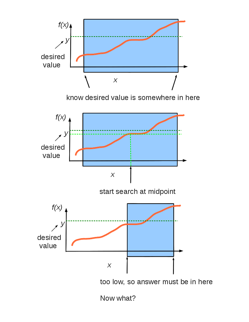 #
# Here is a useful application of binary search.
# ### Effective Branching Factor
# How can we compare the efficiency of different search algorithms, or of
# the A\* algorithm using different heuristic functions? We can use the
# computation time and the maximum amount of memory used during the
# search.
#
# It would also be nice to know how "focused" a search is. If we use a
# perfect heuristic function, we should get a search that won't explore
# any nodes that do not lie on an optimal search path.
#
# A measure related to this is the "effective branching factor". The
# branching factor of a tree is the number of children at each node. If
# this is not the same for all nodes, then we can find an average, or
# "effective" branching factor.
#
# If we do a breadth-first (or depth-first) search on a tree like this
#
#
#
# Here is a useful application of binary search.
# ### Effective Branching Factor
# How can we compare the efficiency of different search algorithms, or of
# the A\* algorithm using different heuristic functions? We can use the
# computation time and the maximum amount of memory used during the
# search.
#
# It would also be nice to know how "focused" a search is. If we use a
# perfect heuristic function, we should get a search that won't explore
# any nodes that do not lie on an optimal search path.
#
# A measure related to this is the "effective branching factor". The
# branching factor of a tree is the number of children at each node. If
# this is not the same for all nodes, then we can find an average, or
# "effective" branching factor.
#
# If we do a breadth-first (or depth-first) search on a tree like this
#
# 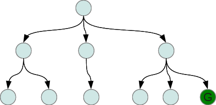 #
# we will have explored 1 + 3 + 6 = 10 nodes. What is the effective
# branching factor for this tree? Or, stated mathematically, what is
# the value of $b$ in
#
# $$ 1 + b + b^2 = 10$$
#
# Now we can solve this for $b$. What should the value be, roughly?
# Solve it exactly. What do you get?
# We can solve this one exactly, but what if the search is 10 levels
# deep? We will have to do a search (yay!) to find the value of $b$.
# How? Could pick a whole bunch of values randomly.....
#
# How about a binary search? To start a binary search we need to pick a
# low and high value of $b$ that we know bracket the true value. For a
# search that explored $n$ nodes to a maximum depth of $d$, what would
# good low and high values be? Now do a binary search between these two
# values and for each new guess at $b$, calculate
#
# $$ 1 + b + b^2 + \cdots + b^d$$
#
# and compare the result with the actual number of nodes, $n$. Use the
# comparison to continue the binary search. Continue until the range of
# possible values of $b$ are within a desired precision, such as $0.01$. A faster way
# to calculate the above quantity is
#
# $$ \frac{1-b^{d+1}}{1-b}$$
#
# How would you derive this?
#
# To estimate the effective branching factor, you could define a
# function `def ebf(numberNodes, depth, precision=0.01)`. Then, to use it
#
#
# In [3]: ebf(100, 12, 0.01)
# Out[3]: 1.3034343719482422
#
# In [4]: ebf(0, 0)
# Out[4]: 0
#
# In [5]: ebf(1, 1,)
# Out[5]: 0.0078125
# ### Run and Twiddle
#
# Take a step in a random direction from current state. If value is
# higher, keep going in that direction. If value is lower, pick a new
# random direction. The "smallest" implementation of this algorithm is
# found in [bacteria](http://www.pnas.org/content/99/1/7.full).
# ### Nelder-Mead Simplex Algorithm
#
# This is not in our text. See the
# [Scholarpedia
# entry for Nelder-Mead](http://www.scholarpedia.org/article/Nelder-Mead_algorithm). This maintains a set of $k$ good states. To
# generate one next state to evaluate, the worst of the $k$ states is
# reflected through the centroid, or mean, of the $k$ states. If the
# new state is better than the worst of the $k$ states, it replaces the
# worst state.
#
# Also see the [Python
# documentation for fmin function in scipy](https://docs.scipy.org/doc/scipy/reference/generated/scipy.optimize.fmin.html).
# ### CMA-ES
#
# Stands for [Covariance
# Matrix Adaptation Evolution Strategy](https://en.wikipedia.org/wiki/CMA-ES). A Gaussian distribution is
# fit to the set of good states and a new state is generated by sampling
# probabilistically from the Gaussian distribution. The Gaussian
# distribution is updated when a new good state is found.
# [Recent
# results show](http://hal.archives-ouvertes.fr/docs/00/17/32/07/PDF/geccodcma.pdf) show that certain quasi-random methods are
# computationally more efficient.
# ## With Derivatives of Value Function
#
# When the derivative of the value function with respect to each
# component of the state can be calculated, then many derivative-based
# searches are available. If you know the slope at the current state,
# you know which direction to go. If you also know the second
# derivative, you can make some intelligent guesses at how far to go.
#
# If the state has multiple components, almost always the case, the
# derivatives are gradients, and the second derivatives are Hessian
# matrices.
# Let's find the minimum of the function
#
# $$f(x) = 2 x^4 + 3 x^3 + 3$$
#
# Its first derivative is
#
# $$\frac{df(x)}{dx} = 8 x^3 + 9 x^2$$
#
# and its second derivative is
#
# $$\frac{d^2f(x)}{dx^2} = 24 x^2 + 18 x$$
#
# In[31]:
import time
import IPython.display as ipd # for display and clear_output
import random
def f(x):
return 2 * x**4 + 3 * x**3 + 3
def df(x):
return 8 * x**3 + 9 * x**2
def ddf(x):
return 24 * x**2 + 18*x
def taylorf(x,dx):
return f(x) + df(x) * dx + 0.5 * ddf(x) * dx**2
xs = np.linspace(-2,1,num=100)
dxs = np.linspace(-0.5,0.5,num=100)
fig = plt.figure(figsize=(18, 8))
for rep in range(5):
x = random.uniform(-2, 1) # first guess at minimum
for step in range(10):
time.sleep(1) # sleep 2 seconds
plt.clf()
plt.plot(xs, f(xs))
plt.grid('on')
plt.plot(x+dxs, taylorf(x, dxs),'g-',linewidth=5, alpha=0.4)
plt.plot(x, f(x), 'ro')
y0, y1 = plt.ylim()
plt.plot([x, x], [y0, y1], 'r--')
if step == 0:
plt.text(x, 10, 'New first x', color='r', fontsize=40)
plt.text(x + 0.05, (y0 + y1) * 0.5, str(x), color='r', fontsize=20)
x = x - df(x) / float(ddf(x))
plt.plot(x, f(x), 'go')
plt.legend(('$f(x)$', '$\hat{f}(x)$'))
ipd.clear_output(wait=True)
ipd.display(fig)
ipd.clear_output(wait=True)
# ### Try these
#
# 4.1 What kind of search do we get from
#
# - Local beam search with $k=1$?
# - Local beam search with one initial state and no limit on the number of states retained?
# - Simulated annealing with $T=0$ at all times?
# - Simulated annealing with $T=\infty$?
# - Genetic algorithm with population size $k=1$?
# - Gradient-ascent in a discrete state and action space?
# - Nelder-Mead with $k=2$ in a two-dimensional state space?
# # On-Line Search Algorithms (from Section 4.5)
#
# For many real-world problems, an agent cannot predict the outcome of
# applying an action in the current state. It must take the action and
# observe the new state.
#
# An agent can end up in a dead-end from which it cannot recover. We
# will ignore this, and assume that a search problem is **safely
# explorable**---some goal state is reachable from every reachable
# state.
#
# An on-line search agent cannot explore the successors to an arbitrary
# node, but only the successors of the current node. This is the nature
# of depth-first so the authors adapt off-line dept-first search to
# an on-line search algorithm. Results of each action are stored in a
# map that associates each state-action pair with the resulting state.
# It assumes it is possible to undo, or reverse, each action in order to
# backtrack.
#
# An on-line version of A* is learning real-time A* , or LRTA*
# Instead of maintaining memory of states as in the above depth-first
# algorithm, LRTA* only maintains a memory of the current best estimate
# of cost to reach a goal for each node. It updates this estimate after
# each action is tried. It assumes it can identify all successors for a
# state and compare their remaining cost estimates. An interesting
# aspect is that all untried actions are assumed to result in a state
# whose heuristic function value is correct, a feature called **optimism
# under uncertainty**.
#
# Learning better estimates of remaining cost based on single steps is
# at the heart of **reinforcement learning**, covered in Chapter 21.
#
# we will have explored 1 + 3 + 6 = 10 nodes. What is the effective
# branching factor for this tree? Or, stated mathematically, what is
# the value of $b$ in
#
# $$ 1 + b + b^2 = 10$$
#
# Now we can solve this for $b$. What should the value be, roughly?
# Solve it exactly. What do you get?
# We can solve this one exactly, but what if the search is 10 levels
# deep? We will have to do a search (yay!) to find the value of $b$.
# How? Could pick a whole bunch of values randomly.....
#
# How about a binary search? To start a binary search we need to pick a
# low and high value of $b$ that we know bracket the true value. For a
# search that explored $n$ nodes to a maximum depth of $d$, what would
# good low and high values be? Now do a binary search between these two
# values and for each new guess at $b$, calculate
#
# $$ 1 + b + b^2 + \cdots + b^d$$
#
# and compare the result with the actual number of nodes, $n$. Use the
# comparison to continue the binary search. Continue until the range of
# possible values of $b$ are within a desired precision, such as $0.01$. A faster way
# to calculate the above quantity is
#
# $$ \frac{1-b^{d+1}}{1-b}$$
#
# How would you derive this?
#
# To estimate the effective branching factor, you could define a
# function `def ebf(numberNodes, depth, precision=0.01)`. Then, to use it
#
#
# In [3]: ebf(100, 12, 0.01)
# Out[3]: 1.3034343719482422
#
# In [4]: ebf(0, 0)
# Out[4]: 0
#
# In [5]: ebf(1, 1,)
# Out[5]: 0.0078125
# ### Run and Twiddle
#
# Take a step in a random direction from current state. If value is
# higher, keep going in that direction. If value is lower, pick a new
# random direction. The "smallest" implementation of this algorithm is
# found in [bacteria](http://www.pnas.org/content/99/1/7.full).
# ### Nelder-Mead Simplex Algorithm
#
# This is not in our text. See the
# [Scholarpedia
# entry for Nelder-Mead](http://www.scholarpedia.org/article/Nelder-Mead_algorithm). This maintains a set of $k$ good states. To
# generate one next state to evaluate, the worst of the $k$ states is
# reflected through the centroid, or mean, of the $k$ states. If the
# new state is better than the worst of the $k$ states, it replaces the
# worst state.
#
# Also see the [Python
# documentation for fmin function in scipy](https://docs.scipy.org/doc/scipy/reference/generated/scipy.optimize.fmin.html).
# ### CMA-ES
#
# Stands for [Covariance
# Matrix Adaptation Evolution Strategy](https://en.wikipedia.org/wiki/CMA-ES). A Gaussian distribution is
# fit to the set of good states and a new state is generated by sampling
# probabilistically from the Gaussian distribution. The Gaussian
# distribution is updated when a new good state is found.
# [Recent
# results show](http://hal.archives-ouvertes.fr/docs/00/17/32/07/PDF/geccodcma.pdf) show that certain quasi-random methods are
# computationally more efficient.
# ## With Derivatives of Value Function
#
# When the derivative of the value function with respect to each
# component of the state can be calculated, then many derivative-based
# searches are available. If you know the slope at the current state,
# you know which direction to go. If you also know the second
# derivative, you can make some intelligent guesses at how far to go.
#
# If the state has multiple components, almost always the case, the
# derivatives are gradients, and the second derivatives are Hessian
# matrices.
# Let's find the minimum of the function
#
# $$f(x) = 2 x^4 + 3 x^3 + 3$$
#
# Its first derivative is
#
# $$\frac{df(x)}{dx} = 8 x^3 + 9 x^2$$
#
# and its second derivative is
#
# $$\frac{d^2f(x)}{dx^2} = 24 x^2 + 18 x$$
#
# In[31]:
import time
import IPython.display as ipd # for display and clear_output
import random
def f(x):
return 2 * x**4 + 3 * x**3 + 3
def df(x):
return 8 * x**3 + 9 * x**2
def ddf(x):
return 24 * x**2 + 18*x
def taylorf(x,dx):
return f(x) + df(x) * dx + 0.5 * ddf(x) * dx**2
xs = np.linspace(-2,1,num=100)
dxs = np.linspace(-0.5,0.5,num=100)
fig = plt.figure(figsize=(18, 8))
for rep in range(5):
x = random.uniform(-2, 1) # first guess at minimum
for step in range(10):
time.sleep(1) # sleep 2 seconds
plt.clf()
plt.plot(xs, f(xs))
plt.grid('on')
plt.plot(x+dxs, taylorf(x, dxs),'g-',linewidth=5, alpha=0.4)
plt.plot(x, f(x), 'ro')
y0, y1 = plt.ylim()
plt.plot([x, x], [y0, y1], 'r--')
if step == 0:
plt.text(x, 10, 'New first x', color='r', fontsize=40)
plt.text(x + 0.05, (y0 + y1) * 0.5, str(x), color='r', fontsize=20)
x = x - df(x) / float(ddf(x))
plt.plot(x, f(x), 'go')
plt.legend(('$f(x)$', '$\hat{f}(x)$'))
ipd.clear_output(wait=True)
ipd.display(fig)
ipd.clear_output(wait=True)
# ### Try these
#
# 4.1 What kind of search do we get from
#
# - Local beam search with $k=1$?
# - Local beam search with one initial state and no limit on the number of states retained?
# - Simulated annealing with $T=0$ at all times?
# - Simulated annealing with $T=\infty$?
# - Genetic algorithm with population size $k=1$?
# - Gradient-ascent in a discrete state and action space?
# - Nelder-Mead with $k=2$ in a two-dimensional state space?
# # On-Line Search Algorithms (from Section 4.5)
#
# For many real-world problems, an agent cannot predict the outcome of
# applying an action in the current state. It must take the action and
# observe the new state.
#
# An agent can end up in a dead-end from which it cannot recover. We
# will ignore this, and assume that a search problem is **safely
# explorable**---some goal state is reachable from every reachable
# state.
#
# An on-line search agent cannot explore the successors to an arbitrary
# node, but only the successors of the current node. This is the nature
# of depth-first so the authors adapt off-line dept-first search to
# an on-line search algorithm. Results of each action are stored in a
# map that associates each state-action pair with the resulting state.
# It assumes it is possible to undo, or reverse, each action in order to
# backtrack.
#
# An on-line version of A* is learning real-time A* , or LRTA*
# Instead of maintaining memory of states as in the above depth-first
# algorithm, LRTA* only maintains a memory of the current best estimate
# of cost to reach a goal for each node. It updates this estimate after
# each action is tried. It assumes it can identify all successors for a
# state and compare their remaining cost estimates. An interesting
# aspect is that all untried actions are assumed to result in a state
# whose heuristic function value is correct, a feature called **optimism
# under uncertainty**.
#
# Learning better estimates of remaining cost based on single steps is
# at the heart of **reinforcement learning**, covered in Chapter 21.