#!/usr/bin/env python
# coding: utf-8
# # Pump systems
#
# A pump is used to move fluid through a pipeline.
#
# 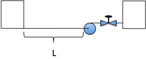 #
# * The flow rate is controlled by a valve.
# * The pump supplies pressure at various flow rates.
# * If we divide the pressure by the fluid density and gravity, which are both constant, we get units of length, which we call a **head**.
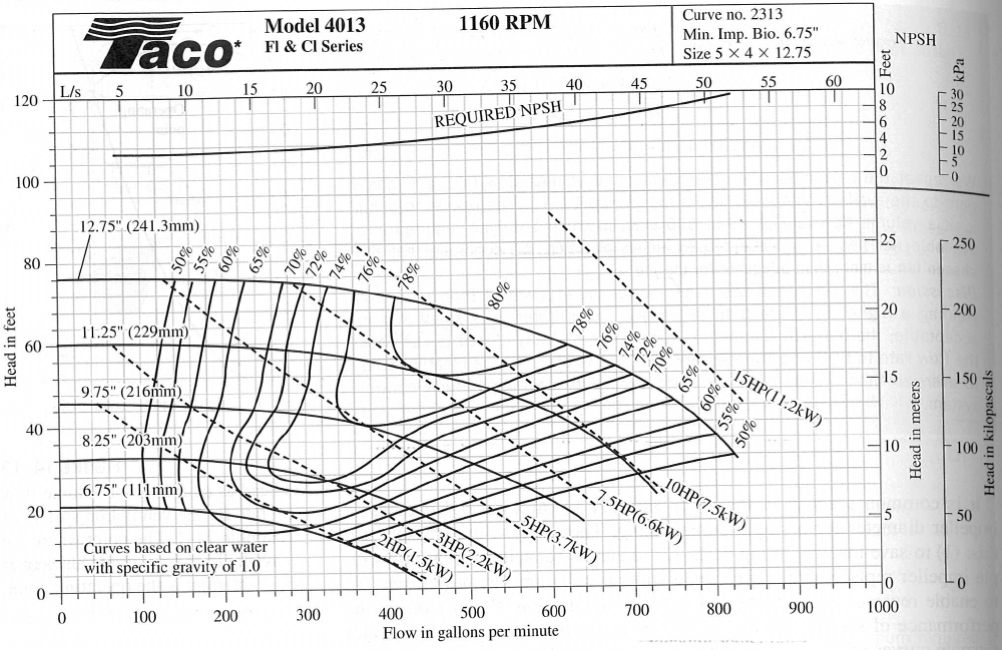
# * So, we can plot **head** versus flow rate. Here's an example of a ***pump curve***
# * We'll consider the 12.75 inch pump size (top curve).
#
#
#
# * The flow rate is controlled by a valve.
# * The pump supplies pressure at various flow rates.
# * If we divide the pressure by the fluid density and gravity, which are both constant, we get units of length, which we call a **head**.
# * So, we can plot **head** versus flow rate. Here's an example of a ***pump curve***
# * We'll consider the 12.75 inch pump size (top curve).
#
#  #
# * The flow through the system is related by a mechanical energy balance:
# $$\frac{\Delta P}{\rho g} + \frac{\Delta v^2}{2g} + \Delta z = h_p -\frac{fLv^2}{2Dg} - \frac{Kv^2}{2g}$$
# * Here, $z$ is height, $f$ is the pipe friction factor, $L$ is the pipe length, $D$ is the pipe diameter, and $K$ is a valve coeficient.
# * We'll assume the tanks are open to the atmosphere, have no vecocity at the top surface, and are at the same height, so that the left hand side is zero. We're assuming no other friction losses besides the pipe and the valve. Rearrange to
#
# $$h_p = \frac{fLv^2}{2Dg} + \frac{Kv^2}{2g}$$.
#
# * The system operates where the **operating curve (equation above)** and the **pump curve** in the figure intersect.
# * That is, the system can operate anywhere on the operative curve (any head/flow combination on that curve), but because the flow is driven by a pump, we are restricted to the points that also lie on the pump curve.
# * We adjust the intersection point, that is, the operating point of the system, by opening or closing the valve (changing $K$). This will effectively pivot the operating curve left or right about the origin.
#
# ## Problem
# * L = 35 m
# * f = 0.015
# * D = 0.1
#
# Develop a widget that will let us find and visualize the operating point by opening/closing the valve (changing $K$).
#
# In[1]:
import numpy as np
import matplotlib.pyplot as plt
get_ipython().run_line_magic('matplotlib', 'inline')
from scipy.interpolate import interp1d
from scipy.optimize import fsolve
import pint; u = pint.UnitRegistry()
import ipywidgets as wg
from IPython.display import display
# ### Part a
#
# Use something like the [web plot digitizer](https://apps.automeris.io/wpd/) to get the pump data. This will give you head versus flow rate. Use pint to convert the units to SI (m, and m$^3$/s), then store the arrays without units for later calculation.
# In[ ]:
# ### Part b
#
# Given the flow/head data from Part a, create a pump curve function using ```interp1d```.
# In[ ]:
# ### Part c
#
# Write a function for the operating curve equation that takes two parameters: the flow rate and the valve coeffient $K$, and returns the required pump head $h$.
#
# In[ ]:
# ### Part d
#
# Write a function that takes $K$ as a parameter and prints the operating point. The function should also plot the operating curve and the pump curve as lines, and the operating point as a single point.
# In[ ]:
# ### Part e
#
# Set your function from Part d to work as an interactive plot with $K$ the parameter that is changed. $K$ should vary from 0 to 1000. Note that low K corresponds to an open valve, and high K corresponds to a closed valve.
# In[ ]:
#
# * The flow through the system is related by a mechanical energy balance:
# $$\frac{\Delta P}{\rho g} + \frac{\Delta v^2}{2g} + \Delta z = h_p -\frac{fLv^2}{2Dg} - \frac{Kv^2}{2g}$$
# * Here, $z$ is height, $f$ is the pipe friction factor, $L$ is the pipe length, $D$ is the pipe diameter, and $K$ is a valve coeficient.
# * We'll assume the tanks are open to the atmosphere, have no vecocity at the top surface, and are at the same height, so that the left hand side is zero. We're assuming no other friction losses besides the pipe and the valve. Rearrange to
#
# $$h_p = \frac{fLv^2}{2Dg} + \frac{Kv^2}{2g}$$.
#
# * The system operates where the **operating curve (equation above)** and the **pump curve** in the figure intersect.
# * That is, the system can operate anywhere on the operative curve (any head/flow combination on that curve), but because the flow is driven by a pump, we are restricted to the points that also lie on the pump curve.
# * We adjust the intersection point, that is, the operating point of the system, by opening or closing the valve (changing $K$). This will effectively pivot the operating curve left or right about the origin.
#
# ## Problem
# * L = 35 m
# * f = 0.015
# * D = 0.1
#
# Develop a widget that will let us find and visualize the operating point by opening/closing the valve (changing $K$).
#
# In[1]:
import numpy as np
import matplotlib.pyplot as plt
get_ipython().run_line_magic('matplotlib', 'inline')
from scipy.interpolate import interp1d
from scipy.optimize import fsolve
import pint; u = pint.UnitRegistry()
import ipywidgets as wg
from IPython.display import display
# ### Part a
#
# Use something like the [web plot digitizer](https://apps.automeris.io/wpd/) to get the pump data. This will give you head versus flow rate. Use pint to convert the units to SI (m, and m$^3$/s), then store the arrays without units for later calculation.
# In[ ]:
# ### Part b
#
# Given the flow/head data from Part a, create a pump curve function using ```interp1d```.
# In[ ]:
# ### Part c
#
# Write a function for the operating curve equation that takes two parameters: the flow rate and the valve coeffient $K$, and returns the required pump head $h$.
#
# In[ ]:
# ### Part d
#
# Write a function that takes $K$ as a parameter and prints the operating point. The function should also plot the operating curve and the pump curve as lines, and the operating point as a single point.
# In[ ]:
# ### Part e
#
# Set your function from Part d to work as an interactive plot with $K$ the parameter that is changed. $K$ should vary from 0 to 1000. Note that low K corresponds to an open valve, and high K corresponds to a closed valve.
# In[ ]: