#!/usr/bin/env python
# coding: utf-8

# In[1]:


get_ipython().run_line_magic('pdb', '1')

import megatest as mt
mt.ut.ipython_setup()

get_ipython().run_line_magic('matplotlib', 'nbagg')

from mtd.models import *
from pts.models import *
from sec.models import *
from matplotlib import pyplot
import alphamax as am
import datetime
import mtd
import numpy as np
import pandas as pd
import pts
import qgrid
import sec
import seaborn as sns

mt.async.IS_MULTIPROCESSING = False


# In[2]:


security = Security.with_name('VIX Index')
hedge    = Security.with_name('SPX Index')

security_prices = security.quote_df()['adj_mark_in_usd'].dropna()
hedge_prices    = hedge.quote_df()['adj_mark_in_usd'].dropna()

beta_df, beta_figures = mt.analysis.kf_beta(
    security_prices = security_prices,
    hedge_prices    = hedge_prices,
    beta_guess      = -3.0,
    fold_count      = 10,
    iterations      = 10,
    with_analysis   = True
)

for figure in beta_figures:
    figure.set_size_inches(12, 9)


# In[3]:


security = Security.with_name('CMCSA US Equity')
hedge    = Security.with_name('CMCSK US Equity')

security_prices = security.quote_df()['adj_mark_in_usd'].dropna()
hedge_prices    = hedge.quote_df()['adj_mark_in_usd'].dropna()

pairs_df, pairs_figures = mt.analysis.kf_beta(
    security_prices = security_prices,
    hedge_prices    = hedge_prices,
    beta_guess      = 1.0,
    fold_count      = 10,
    iterations      = 10,
    with_analysis   = True,
    return_space    = False
)


# # Kalman Filters
# 
# > the fundamental idea is to blend somewhat inaccurate measurements with somewhat inaccurate models of how the systems behaves to get a filtered estimate that is better than either information source by itself

# ## Pros
# - filters out noise
# - predictive
# - adapative with future data
# - does **NOT** require stationary data
# - outputs a distribution for estimates $ (\mu, \sigma) $
# - for a random walk + noise model, it can be shown to be equivalent to a EWMA (exponentially weighted moving average) [[1](https://stats.stackexchange.com/questions/16458/what-is-the-difference-between-kalman-filter-and-moving-average)]
# - can handle missing data
# - [compared to other methods, found to be superior in calculating beta](http://aum.sagepub.com/content/23/1/1.full.pdf)
# 
# ## Cons
# - assumes linear dependencies (although there is a non-linear version)
# - assumes guassian errors
# - computationally is cubic to the size of the state space

# ## Summary
# 
# <img src="http://alphamaximus.com/assets/images/kalman_filters_0.png" alt="Kalman Filters" style="max-width: 500px; max-height: 500px;"/>
# 
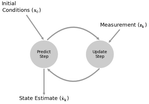# 1. make a prediction from the past
# 2. make a prediction from the observable
# 3. combine estimates

# ## Equations
# 
# $$\begin{align*} 
# x_{t+1} &= Ax_t + Bu_t + w_t \\
# z_t &= Hx_t + v_t \\ 
# \end{align*}$$
# 
# $$\begin{align*} 
# A &= \text{predicion matrix (transition_matrices)} \\
# x &= \text{states} \\
# B &= \text{control matrix (transition_offsets)} \\
# w &= \text{noise (transition_covariance)} \sim N(\theta, Q) \\
# z &= \text{observable readings} \\
# H &= \text{mapping of} \; x \; \text{to observable (observation_matrices)} \\
# v &= \text{observation noise, measurement noise (observation_covariance)} \sim N(\theta, R)
# \end{align*}$$

# ## Best Practices
# - normalize if possible
# - the ratio of $ Q $ and $ R $

# ## Calculating $ Q $
# 
# 1. approximate [[1](https://www.quora.com/How-do-I-determine-the-measurement-noise-in-Kalman-Filter-model)]
#     - calculate variate estimate of error in a controlled environment
#     - if z doesn't change, calculate variance estimate of z
#     - if z does change, calculate variance of regression estimate of z    
# 2. guess
#     - use some constant multiplied by the identity matrix
#     - higher the constant, higher the noise
# 3. MLE
#     - [pykalman](https://github.com/pykalman/pykalman) has an [em](https://pykalman.github.io/#optimizing-parameters) algo
#     - unfortunately, non-convex problem => local optima

# ## Example: Beta

# In[4]:


beta_figures[0]


# ### Equations
# 
# $$ \begin{bmatrix} \beta_{t+1} \\ \alpha_{t+1} \end{bmatrix} = \begin{bmatrix} 1 & 0 \\ 0 & 1 \end{bmatrix} \begin{bmatrix} \beta_{t} \\ \alpha_{t} \end{bmatrix} + \begin{bmatrix} 0 \\ 0 \end{bmatrix} + \begin{bmatrix} w_{\beta, t} \\ w_{\alpha, t} \end{bmatrix} $$
# 
# $$ r_{VIX, t} = \begin{bmatrix} r_{SPX, t} & 1 \end{bmatrix} \begin{bmatrix} \beta_{t} \\ \alpha_{t} \end{bmatrix} + v_t $$

# ### Parameters for [pykalman](https://github.com/pykalman/pykalman)
# 
# #### State Parameters
# 
#     # [beta, alpha] has 2-dimensions
#     n_dim_state = 2
#     
#     # GUESS what is the initial beta/alpha?
#     initial_state_mean = [beta_guess, 0.0]     
#     
#     # GUESS how confident are we for our beta/alpha guesses?
#     initial_state_covariance = np.ones((2, 2)) 
# 

# #### Transition Parameters
# 
#     # how does beta/alpha change over time? random walk!
#     transition_matrices = np.eye(2)
#     
#     # what is the beta/alpha drift over time? random walk!
#     transition_offsets = [0, 0] 
#     
#     # GUESS how much does beta/alpha change due to unmodeled forces?
#     transition_covariance = delta / (1 - delta) * np.eye(2)
# 

# #### Observation Parameters
# 
#     # VIX returns are 1-dimensional
#     n_dim_obs = 1
#     
#     # how do we convert beta/alpha to VIX returns
#     observation_matrices = np.expand_dims(
#         a    = np.vstack([[x], [np.ones(len(x))]]).T,
#         axis = 1
#     ) 
#     
#     # GUESS how much does VIX returns deviate outside of beta/alpha estimates
#     observation_covariance = .01 

# ### Calculate Q and R
# 
# 1. split into k folds
# 2. calculate MSE using pykalman's `em` on previous folds
# 
#         kf.em(
#             X       = y_training,
#             n_iter  = 10,
#             em_vars = ['transition_covariance', 'observation_covariance']
#         )
# 
# 3. use MSE in current fold
# 
# <img src="https://blog.quantopian.com/wp-content/uploads/2012/07/iterative-img.png" alt="walk forward optimization" style="max-width: 500px; max-height: 500px;"/>

# In[5]:


beta_figures[1]


# In[6]:


beta_df.dropna(inplace=True)

resid_kf  = beta_df['beta'] * beta_df['x'] - beta_df['y']
resid_30  = beta_df['beta_30'] * beta_df['x'] - beta_df['y']
resid_250 = beta_df['beta_250'] * beta_df['x'] - beta_df['y']
resid_500 = beta_df['beta_500'] * beta_df['x'] - beta_df['y']

print np.sum(resid_kf**2) / len(resid_kf)
print np.sum(resid_30**2) / len(resid_30)
print np.sum(resid_250**2) / len(resid_250)
print np.sum(resid_500**2) / len(resid_500)


# In[7]:


resid_kf  = beta_df['beta'].shift(1) * beta_df['x'] - beta_df['y']
resid_30  = beta_df['beta_30'].shift(1) * beta_df['x'] - beta_df['y']
resid_250 = beta_df['beta_250'].shift(1) * beta_df['x'] - beta_df['y']
resid_500 = beta_df['beta_500'].shift(1) * beta_df['x'] - beta_df['y']

print np.sum(resid_kf**2) / len(resid_kf)
print np.sum(resid_30**2) / len(resid_30)
print np.sum(resid_250**2) / len(resid_250)
print np.sum(resid_500**2) / len(resid_500)


# In[8]:


beta_figures[2]


# ## Example: Pairs Trading
# 
# $$ \begin{bmatrix} \beta_{t+1} \\ \alpha_{t+1} \end{bmatrix} = \begin{bmatrix} 1 & 0 \\ 0 & 1 \end{bmatrix} \begin{bmatrix} \beta_{t} \\ \alpha_{t} \end{bmatrix} + \begin{bmatrix} 0 \\ 0 \end{bmatrix} + \begin{bmatrix} w_{\beta, t} \\ w_{\alpha, t} \end{bmatrix} $$
# 
# $$ p_{B, t} = \begin{bmatrix} p_{A, t} & 1 \end{bmatrix} \begin{bmatrix} \beta_{t} \\ \alpha_{t} \end{bmatrix} + v_t $$

# In[9]:


pairs_figures[0]


# In[10]:


pairs_figures[1]


# In[11]:


pairs_figures[2]


# ## Unscented Kalman Filter (UKF)
# 
# ### Pros
# - doesn't require linear system
# - doesn't require Gaussian normal noise (with limitations)
# - as computationally complex as standard Kalman filter
# 
# ### Cons
# - no MSE for parameters
# - questionable performance

# ## Equations
# 
# $$
# \begin{align*} 
# x_{t+1} & =  f(x_t, w_t) \\
# z_t & = g(x_t, v_t)
# \end{align*}
# $$
#     
# f = predicion matrix (`transition_functions`)  
# x = states   
# w = noise ~ N(0, Q) (`transition_covariance`)  
# z = observable readings  
# g = mapping of x to observable (`observation_functions`)  
# v = observation noise, measurement noise ~ N(0, R) (`observation_covariance`)

# ## Example: Stochastic Volatility
# 
# $$ r_t = \mu + \sqrt{\nu_t} \, w_t $$
# 
# $$ \nu_{t+1} = \nu_{t} + \theta \, (\omega-\nu_t) + \xi \, \nu_t^{\kappa} \, b_t $$
# 
# where $ w_t $ and $ b_t $ are correlated with a value of $ \rho $.
# 
# For Heston, $ k = 0.5 $ . For GARCH, $ k = 1.0 $. For 3/2, $ k = 1.5 $.
# 
# Let:
# 
# $$ z_t = \frac{1}{\sqrt{1 - \rho^{2}}} (b_t - \rho w_t)$$
# 
# $ z_t $ and $ w_t $ are not correlated!
# 
# $$ w_t = \frac{ r_t - \mu }{ \sqrt{\nu_t} } $$
# 
# $$ b_t = \sqrt{1 - \rho^{2}} \,  z_t + \rho w_t $$
# 
# $$ b_t = \sqrt{1 - \rho^{2}} \,  z_t + \rho \frac{ r_t - \mu }{ \sqrt{\nu_t} } $$
# 
# Finally...
# 
# $$ \nu_{t+1} = \nu_{t} + \theta \, (\omega-\nu_t) + \xi \, \nu_t^{\kappa} \left [ \sqrt{1 - \rho^{2}} \,  z_t + \rho \frac{ r_t - \mu }{ \sqrt{\nu_t} } \right ] $$
# 
# $$ r_t = \mu + \sqrt{\nu_t} w_t $$

# In[12]:


def sv_kf_functions(mu, theta, omega, xi, k, rho, log_returns):

    def f(current_state, transition_noise, log_return):
        b_t = math.sqrt(1 - rho ** 2) * transition_noise + rho * (r - mu) / math.sqrt(current_state)
        return current_state + theta * (omega - current_state) + xi * current_state ** k * b_t

    def g(current_state, observation_noise):
        return mu + math.sqrt(current_state) * observation_noise
    
    return [partial(f, log_return=log_return) for log_return in log_returns], g


# ## References
# - [Quantopian Video](https://www.quantopian.com/posts/quantopian-lecture-series-kalman-filters)
# - [Quantopian Notebook](https://www.quantopian.com/posts/quantopian-lecture-series-kalman-filters)
# - [pykalman Documentation](https://pykalman.github.io/)
# - [Concept](http://www.bzarg.com/p/how-a-kalman-filter-works-in-pictures/)
# - [Equations](http://greg.czerniak.info/guides/kalman1/)
# - [Beta Example](http://www.thealgoengineer.com/2014/online_linear_regression_kalman_filter/)
# - [Numerical Example](http://bilgin.esme.org/BitsBytes/KalmanFilterforDummies.aspx)
# - [Stochastic Volatility Example](https://www.cis.upenn.edu/~mkearns/finread/filtering_in_finance.pdf)
# - [A Textbook](http://www.cs.unc.edu/~tracker/media/pdf/SIGGRAPH2001_CoursePack_08.pdf)
# - [An IPython Textbook](https://github.com/rlabbe/Kalman-and-Bayesian-Filters-in-Python/blob/master/01-g-h-filter.ipynb)

# <img src="http://alphamaximus.com/assets/images/profile.png" alt="JPN" style="width: 100px;"/>
# 
# ## About Me
# 
# I'm a trader/quant.  
# I started blogging on [Alphamaximus](http://alphamaximus.com)  
# I'm also a co-founder of [Bonjournal](https://bonjourn.al).
# 
# Follow me on [Twitter](https://twitter.com/_jonathanng_).