 #
# * pip install patsy pandas
# * pip install pymc - PyMC2
# * pip install git+https://github.com/pymc-devs/pymc3 - PyMC3
# * Also need Scipy, NumPy, Seaborn - basically the PyData Stack
# * Anaconda is excellent to get up and running
# * Stop me and ask questions as we go along
#
# # Newsflash
# * PyMC3 is Beta
# * Big shout out to John Salvatier, Thomas Wiecki and Chris Fonnesbeck - great work people :)
# * You are attending the first tutorial in the world on PyMC3 since it went Beta!
# * Welcome to the cutting-edge of Probabilistic Programming with the PyData stack :)
#
# * The next slide is just some code. Run it as a test for if you've installed the correct things.
# * The code is taken from Thomas Wiecki's tutorials on applying PyMC3 to Quantitative finance
# In[31]:
get_ipython().run_line_magic('matplotlib', 'inline')
#Most of this code is from @twiecki - used with attribution
import pandas as pd
import seaborn as sns
import matplotlib.pyplot as plt
import numpy as np
import itertools
import scipy as sp
import pymc3 as pm3
import theano.tensor as T
from scipy import stats
from IPython.core.pylabtools import figsize
figsize(12, 12)
sns.set_style('darkgrid')
import scipy
data_0 = pd.read_csv('data0.csv', index_col=0, parse_dates=True, header=None)[1]
data_1 = pd.read_csv('data1.csv', index_col=0, parse_dates=True, header=None)[1]
def var_cov_var_t(P, c, nu=1, mu=0, sigma=1, **kwargs):
"""
Variance-Covariance calculation of daily Value-at-Risk
using confidence level c, with mean of returns mu
and standard deviation of returns sigma, on a portfolio
of value P.
"""
alpha = stats.t.ppf(1-c, nu, mu, sigma)
return P - P*(alpha + 1)
def var_cov_var_normal(P, c, mu=0, sigma=1, **kwargs):
"""
Variance-Covariance calculation of daily Value-at-Risk
using confidence level c, with mean of returns mu
and standard deviation of returns sigma, on a portfolio
of value P.
"""
alpha = stats.norm.ppf(1-c, mu, sigma)
return P - P*(alpha + 1)
def sample_normal(mu=0, sigma=1, **kwargs):
samples = stats.norm.rvs(mu, sigma, kwargs.get('size', 100))
return samples
def sample_t(nu=1, mu=0, sigma=1, **kwargs):
samples = stats.t.rvs(nu, mu, sigma, kwargs.get('size', 100))
return samples
def eval_normal(mu=0, sigma=1, **kwargs):
pdf = stats.norm(mu, sigma).pdf(kwargs.get('x', np.linspace(-0.05, 0.05, 500)))
return pdf
def eval_t(nu=1, mu=0, sigma=1, **kwargs):
samples = stats.t(nu, mu, sigma).pdf(kwargs.get('x', np.linspace(-0.05, 0.05, 500)))
return samples
def logp_normal(mu=0, sigma=1, **kwargs):
logp = np.sum(stats.norm(mu, sigma).logpdf(kwargs['data']))
return logp
def logp_t(nu=1, mu=0, sigma=1, **kwargs):
logp = np.sum(stats.t(nu, mu, sigma).logpdf(kwargs['data']))
return logp
# generate posterior predictive
def post_pred(func, trace, *args, **kwargs):
samples = kwargs.pop('samples', 50)
ppc = []
for i, idx in enumerate(np.linspace(0, len(trace), samples)):
t = trace[int(i)]
try:
kwargs['nu'] = t['nu_minus_one']+1
except KeyError:
pass
mu = t['mean returns']
sigma = t['volatility']
ppc.append(func(*args, mu=mu, sigma=sigma, **kwargs))
return ppc
def plot_strats(sharpe=False):
figsize(12, 6)
f, (ax1, ax2) = plt.subplots(1, 2)
if sharpe:
label = 'etrade\nn=%i\nSharpe=%.2f' % (len(data_0), (data_0.mean() / data_0.std() * np.sqrt(252)))
else:
label = 'etrade\nn=%i\n' % (len(data_0))
sns.distplot(data_0, kde=False, ax=ax1, label=label, color='b')
ax1.set_xlabel('daily returns'); ax1.legend(loc=0)
if sharpe:
label = 'IB\nn=%i\nSharpe=%.2f' % (len(data_1), (data_1.mean() / data_1.std() * np.sqrt(252)))
else:
label = 'IB\nn=%i\n' % (len(data_1))
sns.distplot(data_1, kde=False, ax=ax2, label=label, color='g')
ax2.set_xlabel('daily returns'); ax2.legend(loc=0);
# In[33]:
def model_returns_normal(data):
with pm3.Model() as model:
mu = pm3.Normal('mean returns', mu=0, sd=.01, testval=data.mean())
sigma, log_sigma = model.TransformedVar('volatility',
pm3.HalfCauchy.dist(beta=1, testval=data.std()),
pm3.transforms.logtransform)
#sigma = pm.HalfCauchy('volatility', beta=.1, testval=data.std())
returns = pm3.Normal('returns', mu=mu, sd=sigma, observed=data)
ann_vol = pm3.Deterministic('annual volatility', returns.distribution.variance**.5 * np.sqrt(252))
sharpe = pm3.Deterministic('sharpe',
returns.distribution.mean / returns.distribution.variance**.5 * np.sqrt(252))
start = pm3.find_MAP(fmin=scipy.optimize.fmin_powell)
step = pm3.NUTS(scaling=start)
trace_normal = pm3.sample(5000, step, start=start)
return trace_normal
def model_returns_t(data):
with pm3.Model() as model:
mu = pm3.Normal('mean returns', mu=0, sd=.01, testval=data.mean())
sigma, log_sigma = model.TransformedVar('volatility',
pm3.HalfCauchy.dist(beta=1, testval=data.std()),
pm3.transforms.logtransform)
nu, log_nu = model.TransformedVar('nu_minus_one',
pm3.Exponential.dist(1./10., testval=3.),
pm3.transforms.logtransform)
returns = pm3.T('returns', nu=nu+2, mu=mu, sd=sigma, observed=data)
ann_vol = pm3.Deterministic('annual volatility', returns.distribution.variance**.5 * np.sqrt(252))
sharpe = pm3.Deterministic('sharpe',
returns.distribution.mean / returns.distribution.variance**.5 * np.sqrt(252))
start = pm3.find_MAP(fmin=scipy.optimize.fmin_powell)
step = pm3.NUTS(scaling=start)
trace = pm3.sample(5000, step, start=start)
return trace
def model_returns_t_stoch_vol(data):
from pymc3.distributions.timeseries import GaussianRandomWalk
with pm3.Model() as model:
mu = pm3.Normal('mean returns', mu=0, sd=.01, testval=data.mean())
step_size, log_step_size = model.TransformedVar('step size',
pm3.Exponential.dist(1./.02, testval=.06),
pm3.transforms.logtransform)
vol = GaussianRandomWalk('volatility', step_size**-2, shape=len(data))
nu, log_nu = model.TransformedVar('nu_minus_one',
pm3.Exponential.dist(1./10., testval=3.),
pm3.transforms.logtransform)
returns = pm3.T('returns', nu=nu+2, mu=mu, lam=pm.exp(-2*vol), observed=data)
#ann_vol = pm.Deterministic('annual volatility', returns.distribution.variance**.5 * np.sqrt(252))
#sharpe = pm.Deterministic('sharpe',
# returns.distribution.mean / ann_vol)
start = pm3.find_MAP(vars=[vol], fmin=sp.optimize.fmin_l_bfgs_b)
#start = pm.find_MAP(fmin=scipy.optimize.fmin_powell, start=start)
step = pm3.NUTS(scaling=start)
trace = pm3.sample(5000, step, start=start)
return trace
results_normal = {0: model_returns_normal(data_0),
1: model_returns_normal(data_1)}
results_t = {0: model_returns_t(data_0),
1: model_returns_t(data_1)}
# ##Who am I?
# * I'm a Data Analytics Professional based in Luxembourg
# * I currently work for Vodafone
# * My intellectual background is in Physics, Philosophy and Mathematics - including some Financial Mathematics
# * I worked at Amazon in Supply Chain Analytics
# * I interned at http://import.io - where I got introduced to Data Science
# * I've made open source contributions to Pandas and Probabilistic Programming and Bayesian Methods for Hackers.
# * All opinions are my own!
#
#
#
# * pip install patsy pandas
# * pip install pymc - PyMC2
# * pip install git+https://github.com/pymc-devs/pymc3 - PyMC3
# * Also need Scipy, NumPy, Seaborn - basically the PyData Stack
# * Anaconda is excellent to get up and running
# * Stop me and ask questions as we go along
#
# # Newsflash
# * PyMC3 is Beta
# * Big shout out to John Salvatier, Thomas Wiecki and Chris Fonnesbeck - great work people :)
# * You are attending the first tutorial in the world on PyMC3 since it went Beta!
# * Welcome to the cutting-edge of Probabilistic Programming with the PyData stack :)
#
# * The next slide is just some code. Run it as a test for if you've installed the correct things.
# * The code is taken from Thomas Wiecki's tutorials on applying PyMC3 to Quantitative finance
# In[31]:
get_ipython().run_line_magic('matplotlib', 'inline')
#Most of this code is from @twiecki - used with attribution
import pandas as pd
import seaborn as sns
import matplotlib.pyplot as plt
import numpy as np
import itertools
import scipy as sp
import pymc3 as pm3
import theano.tensor as T
from scipy import stats
from IPython.core.pylabtools import figsize
figsize(12, 12)
sns.set_style('darkgrid')
import scipy
data_0 = pd.read_csv('data0.csv', index_col=0, parse_dates=True, header=None)[1]
data_1 = pd.read_csv('data1.csv', index_col=0, parse_dates=True, header=None)[1]
def var_cov_var_t(P, c, nu=1, mu=0, sigma=1, **kwargs):
"""
Variance-Covariance calculation of daily Value-at-Risk
using confidence level c, with mean of returns mu
and standard deviation of returns sigma, on a portfolio
of value P.
"""
alpha = stats.t.ppf(1-c, nu, mu, sigma)
return P - P*(alpha + 1)
def var_cov_var_normal(P, c, mu=0, sigma=1, **kwargs):
"""
Variance-Covariance calculation of daily Value-at-Risk
using confidence level c, with mean of returns mu
and standard deviation of returns sigma, on a portfolio
of value P.
"""
alpha = stats.norm.ppf(1-c, mu, sigma)
return P - P*(alpha + 1)
def sample_normal(mu=0, sigma=1, **kwargs):
samples = stats.norm.rvs(mu, sigma, kwargs.get('size', 100))
return samples
def sample_t(nu=1, mu=0, sigma=1, **kwargs):
samples = stats.t.rvs(nu, mu, sigma, kwargs.get('size', 100))
return samples
def eval_normal(mu=0, sigma=1, **kwargs):
pdf = stats.norm(mu, sigma).pdf(kwargs.get('x', np.linspace(-0.05, 0.05, 500)))
return pdf
def eval_t(nu=1, mu=0, sigma=1, **kwargs):
samples = stats.t(nu, mu, sigma).pdf(kwargs.get('x', np.linspace(-0.05, 0.05, 500)))
return samples
def logp_normal(mu=0, sigma=1, **kwargs):
logp = np.sum(stats.norm(mu, sigma).logpdf(kwargs['data']))
return logp
def logp_t(nu=1, mu=0, sigma=1, **kwargs):
logp = np.sum(stats.t(nu, mu, sigma).logpdf(kwargs['data']))
return logp
# generate posterior predictive
def post_pred(func, trace, *args, **kwargs):
samples = kwargs.pop('samples', 50)
ppc = []
for i, idx in enumerate(np.linspace(0, len(trace), samples)):
t = trace[int(i)]
try:
kwargs['nu'] = t['nu_minus_one']+1
except KeyError:
pass
mu = t['mean returns']
sigma = t['volatility']
ppc.append(func(*args, mu=mu, sigma=sigma, **kwargs))
return ppc
def plot_strats(sharpe=False):
figsize(12, 6)
f, (ax1, ax2) = plt.subplots(1, 2)
if sharpe:
label = 'etrade\nn=%i\nSharpe=%.2f' % (len(data_0), (data_0.mean() / data_0.std() * np.sqrt(252)))
else:
label = 'etrade\nn=%i\n' % (len(data_0))
sns.distplot(data_0, kde=False, ax=ax1, label=label, color='b')
ax1.set_xlabel('daily returns'); ax1.legend(loc=0)
if sharpe:
label = 'IB\nn=%i\nSharpe=%.2f' % (len(data_1), (data_1.mean() / data_1.std() * np.sqrt(252)))
else:
label = 'IB\nn=%i\n' % (len(data_1))
sns.distplot(data_1, kde=False, ax=ax2, label=label, color='g')
ax2.set_xlabel('daily returns'); ax2.legend(loc=0);
# In[33]:
def model_returns_normal(data):
with pm3.Model() as model:
mu = pm3.Normal('mean returns', mu=0, sd=.01, testval=data.mean())
sigma, log_sigma = model.TransformedVar('volatility',
pm3.HalfCauchy.dist(beta=1, testval=data.std()),
pm3.transforms.logtransform)
#sigma = pm.HalfCauchy('volatility', beta=.1, testval=data.std())
returns = pm3.Normal('returns', mu=mu, sd=sigma, observed=data)
ann_vol = pm3.Deterministic('annual volatility', returns.distribution.variance**.5 * np.sqrt(252))
sharpe = pm3.Deterministic('sharpe',
returns.distribution.mean / returns.distribution.variance**.5 * np.sqrt(252))
start = pm3.find_MAP(fmin=scipy.optimize.fmin_powell)
step = pm3.NUTS(scaling=start)
trace_normal = pm3.sample(5000, step, start=start)
return trace_normal
def model_returns_t(data):
with pm3.Model() as model:
mu = pm3.Normal('mean returns', mu=0, sd=.01, testval=data.mean())
sigma, log_sigma = model.TransformedVar('volatility',
pm3.HalfCauchy.dist(beta=1, testval=data.std()),
pm3.transforms.logtransform)
nu, log_nu = model.TransformedVar('nu_minus_one',
pm3.Exponential.dist(1./10., testval=3.),
pm3.transforms.logtransform)
returns = pm3.T('returns', nu=nu+2, mu=mu, sd=sigma, observed=data)
ann_vol = pm3.Deterministic('annual volatility', returns.distribution.variance**.5 * np.sqrt(252))
sharpe = pm3.Deterministic('sharpe',
returns.distribution.mean / returns.distribution.variance**.5 * np.sqrt(252))
start = pm3.find_MAP(fmin=scipy.optimize.fmin_powell)
step = pm3.NUTS(scaling=start)
trace = pm3.sample(5000, step, start=start)
return trace
def model_returns_t_stoch_vol(data):
from pymc3.distributions.timeseries import GaussianRandomWalk
with pm3.Model() as model:
mu = pm3.Normal('mean returns', mu=0, sd=.01, testval=data.mean())
step_size, log_step_size = model.TransformedVar('step size',
pm3.Exponential.dist(1./.02, testval=.06),
pm3.transforms.logtransform)
vol = GaussianRandomWalk('volatility', step_size**-2, shape=len(data))
nu, log_nu = model.TransformedVar('nu_minus_one',
pm3.Exponential.dist(1./10., testval=3.),
pm3.transforms.logtransform)
returns = pm3.T('returns', nu=nu+2, mu=mu, lam=pm.exp(-2*vol), observed=data)
#ann_vol = pm.Deterministic('annual volatility', returns.distribution.variance**.5 * np.sqrt(252))
#sharpe = pm.Deterministic('sharpe',
# returns.distribution.mean / ann_vol)
start = pm3.find_MAP(vars=[vol], fmin=sp.optimize.fmin_l_bfgs_b)
#start = pm.find_MAP(fmin=scipy.optimize.fmin_powell, start=start)
step = pm3.NUTS(scaling=start)
trace = pm3.sample(5000, step, start=start)
return trace
results_normal = {0: model_returns_normal(data_0),
1: model_returns_normal(data_1)}
results_t = {0: model_returns_t(data_0),
1: model_returns_t(data_1)}
# ##Who am I?
# * I'm a Data Analytics Professional based in Luxembourg
# * I currently work for Vodafone
# * My intellectual background is in Physics, Philosophy and Mathematics - including some Financial Mathematics
# * I worked at Amazon in Supply Chain Analytics
# * I interned at http://import.io - where I got introduced to Data Science
# * I've made open source contributions to Pandas and Probabilistic Programming and Bayesian Methods for Hackers.
# * All opinions are my own!
#
# # #
| # # | ## peadarcoyle@gmail.com # |
| # # # # | # http://github.com/springcoil # # |
| # # # | # https://www.linkedin.com/in/peadarcoyle # # |
| # # # | # @springcoil # # |
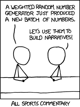 # * Attribution: Xkcd
#
# # How can statistics help with sports?
# * Well fundamentally a Rugby game is a simulatable event.
# * How do we generate a model to predict the outcome of a tournament?
# * How do we quantify our uncertainty in our model?
#
# #What influenced me on this?
#
# * Attribution: Xkcd
#
# # How can statistics help with sports?
# * Well fundamentally a Rugby game is a simulatable event.
# * How do we generate a model to predict the outcome of a tournament?
# * How do we quantify our uncertainty in our model?
#
# #What influenced me on this?
#  # Attribution: Quantopian blog
# #What's wrong with statistics
# * Models should not be built for mathematical convenience (e.g. normality assumption), but to most accurately model the data.
#
# * Pre-specified models, like frequentist statistics, make many assumptions that are all to easily violated.
#
#
# #"The purpose of computation is insight, not numbers." -- Richard Hamming
# # What is Bayesian Statistics?
# * At the core: formula to update our beliefs after having observed data (Bayes formula)
# * Implies that we have a prior belief about the world.
# * Updated beliefs after observing data is called posterior.
# * Beliefs are represented using random variables.
# # Who uses Bayesian Statistics?
# * In the **real** world?
#
# Attribution: Quantopian blog
# #What's wrong with statistics
# * Models should not be built for mathematical convenience (e.g. normality assumption), but to most accurately model the data.
#
# * Pre-specified models, like frequentist statistics, make many assumptions that are all to easily violated.
#
#
# #"The purpose of computation is insight, not numbers." -- Richard Hamming
# # What is Bayesian Statistics?
# * At the core: formula to update our beliefs after having observed data (Bayes formula)
# * Implies that we have a prior belief about the world.
# * Updated beliefs after observing data is called posterior.
# * Beliefs are represented using random variables.
# # Who uses Bayesian Statistics?
# * In the **real** world?
#  # # A Toy Problem
# * A 'toy' problem is a notion from Physics, that you use a simple problem first to derive insight.
# * We will use one of Allen Downeys examples - the code is in PyMC2 and comes from Cameron Davidson-Pilon
# * It is hard to find examples online that aren't influenced by either of these two heavyweights :)
# # First build the model then Infer.
# * Our first step is to build the model.
# * The second step is to infer.
# In the final match of the 2014 FIFA World Cup, Germany defeated Argentina 1-0. How much evidence does this victory provide that Germany had the better team? What is the probability that Germany would win a rematch?
# - From Allen Downey
# Our first step is that we need to make some Modelling decisions
# * What kind of Model suits Football (Soocer)?
# * Well we know empirically that scoring follows a Poisson process
# * This means that a *Poisson* distribution will be our likelihood function
# "Scoring in games like soccer and hockey can be well modeled by a Poisson process, which assumes that each team,
# against a given opponent, will score goals at some goal-scoring rate, $\lambda$, and that this rate is stationary;
# in other words, the probability of scoring a goal is about the same at any point during the game." - Allen Downey
#
# * A good framework for this is to use Bayesian Statistics
# * We will use this in this example - and the code comes from Cameron Davidson-Pilon
#
# In[119]:
import pymc as pm
get_ipython().run_line_magic('matplotlib', 'inline')
sns.set_style("darkgrid")
from matplotlib.pyplot import *
figsize(12,8)
# In[118]:
avg_goals_per_team = 1.34
duration_of_game = 93.
# In[120]:
german_prior = pm.Exponential('german_prior', duration_of_game/avg_goals_per_team)
arg_prior = pm.Exponential('arg_prior', duration_of_game/avg_goals_per_team)
sample = np.array([german_prior.random() for i in range(10000)])
hist(sample, bins=30, normed=True, histtype='stepfilled');
plt.title('Prior distribution: Exponential with mean equal to observed mean');
# * So now that we've done our Prior Distribution. We need to add some observed data and infer our Posterior.
# * Our posterior is 'the probability of winning the final' or the 'what is the most likely result'
# * We model the scoring function as a Poisson taking into account the Prior of the team and the observed data
# * Finally we create a predictive model - which consists of the duration of the game*the prior
# In[40]:
germany = pm.Poisson('germany_obs', german_prior, observed=True, value=[1])
argentina = pm.Poisson('arg_obs', arg_prior, observed=True, value=[0])
germany_predictive = pm.Poisson('germany_predictive', duration_of_game*german_prior)
arg_predictive = pm.Poisson('arg_predictive', duration_of_game*arg_prior)
# In[41]:
mcmc = pm.MCMC([germany, argentina, german_prior,
arg_prior, germany_predictive, arg_predictive])
# * Now we need to run the model :)
# In[42]:
mcmc.sample(20000, 5000)
# In[43]:
german_lambda_trace = mcmc.trace('german_prior')[:]
arg_lambda_trace = mcmc.trace('arg_prior')[:]
# In[121]:
hist(german_lambda_trace, bins=45, histtype='stepfilled', label='Germany',
alpha=0.9, normed=True);
hist(arg_lambda_trace, bins=45, histtype='stepfilled', label='Argentina',
alpha=0.8, normed=True);
plt.legend();
plt.title('Posteriors of average goals/minute of the two teams');
# In[45]:
german_post_trace = mcmc.trace('germany_predictive')[:]
arg_post_trace = mcmc.trace('arg_predictive')[:]
# In[122]:
hist(german_post_trace, bins=10, histtype='stepfilled', label='Germany', alpha=0.9, normed=True);
hist(arg_post_trace, bins=10, histtype='stepfilled', label='Argentina', alpha=0.8, normed=True);
plt.legend();
plt.title('Posteriors of Goals per Team for a 93 minute game');
plt.ylabel('probability')
plt.xlabel('Number of goals')
# In[123]:
print("Probability of Germany winning: %.3f"%(german_post_trace > arg_post_trace).mean())
print("Probability of Argentina winning: %.3f"%(german_post_trace < arg_post_trace).mean())
print("Probability of tie: %.3f"%(german_post_trace == arg_post_trace).mean())
# # Wrap up
# * We built a model of the 'teams strength' from our priors and our knowledge of scoring functions in Soccer.
# * We can definitely apply this kind of formulation to OTHER problems
# * Such as Rugby!
# * Well done you just built a Probabilistic Programming Model :)
# ###So what problem could I apply Bayesian models to?
# * Rugby Analysis!
#
# # A Toy Problem
# * A 'toy' problem is a notion from Physics, that you use a simple problem first to derive insight.
# * We will use one of Allen Downeys examples - the code is in PyMC2 and comes from Cameron Davidson-Pilon
# * It is hard to find examples online that aren't influenced by either of these two heavyweights :)
# # First build the model then Infer.
# * Our first step is to build the model.
# * The second step is to infer.
# In the final match of the 2014 FIFA World Cup, Germany defeated Argentina 1-0. How much evidence does this victory provide that Germany had the better team? What is the probability that Germany would win a rematch?
# - From Allen Downey
# Our first step is that we need to make some Modelling decisions
# * What kind of Model suits Football (Soocer)?
# * Well we know empirically that scoring follows a Poisson process
# * This means that a *Poisson* distribution will be our likelihood function
# "Scoring in games like soccer and hockey can be well modeled by a Poisson process, which assumes that each team,
# against a given opponent, will score goals at some goal-scoring rate, $\lambda$, and that this rate is stationary;
# in other words, the probability of scoring a goal is about the same at any point during the game." - Allen Downey
#
# * A good framework for this is to use Bayesian Statistics
# * We will use this in this example - and the code comes from Cameron Davidson-Pilon
#
# In[119]:
import pymc as pm
get_ipython().run_line_magic('matplotlib', 'inline')
sns.set_style("darkgrid")
from matplotlib.pyplot import *
figsize(12,8)
# In[118]:
avg_goals_per_team = 1.34
duration_of_game = 93.
# In[120]:
german_prior = pm.Exponential('german_prior', duration_of_game/avg_goals_per_team)
arg_prior = pm.Exponential('arg_prior', duration_of_game/avg_goals_per_team)
sample = np.array([german_prior.random() for i in range(10000)])
hist(sample, bins=30, normed=True, histtype='stepfilled');
plt.title('Prior distribution: Exponential with mean equal to observed mean');
# * So now that we've done our Prior Distribution. We need to add some observed data and infer our Posterior.
# * Our posterior is 'the probability of winning the final' or the 'what is the most likely result'
# * We model the scoring function as a Poisson taking into account the Prior of the team and the observed data
# * Finally we create a predictive model - which consists of the duration of the game*the prior
# In[40]:
germany = pm.Poisson('germany_obs', german_prior, observed=True, value=[1])
argentina = pm.Poisson('arg_obs', arg_prior, observed=True, value=[0])
germany_predictive = pm.Poisson('germany_predictive', duration_of_game*german_prior)
arg_predictive = pm.Poisson('arg_predictive', duration_of_game*arg_prior)
# In[41]:
mcmc = pm.MCMC([germany, argentina, german_prior,
arg_prior, germany_predictive, arg_predictive])
# * Now we need to run the model :)
# In[42]:
mcmc.sample(20000, 5000)
# In[43]:
german_lambda_trace = mcmc.trace('german_prior')[:]
arg_lambda_trace = mcmc.trace('arg_prior')[:]
# In[121]:
hist(german_lambda_trace, bins=45, histtype='stepfilled', label='Germany',
alpha=0.9, normed=True);
hist(arg_lambda_trace, bins=45, histtype='stepfilled', label='Argentina',
alpha=0.8, normed=True);
plt.legend();
plt.title('Posteriors of average goals/minute of the two teams');
# In[45]:
german_post_trace = mcmc.trace('germany_predictive')[:]
arg_post_trace = mcmc.trace('arg_predictive')[:]
# In[122]:
hist(german_post_trace, bins=10, histtype='stepfilled', label='Germany', alpha=0.9, normed=True);
hist(arg_post_trace, bins=10, histtype='stepfilled', label='Argentina', alpha=0.8, normed=True);
plt.legend();
plt.title('Posteriors of Goals per Team for a 93 minute game');
plt.ylabel('probability')
plt.xlabel('Number of goals')
# In[123]:
print("Probability of Germany winning: %.3f"%(german_post_trace > arg_post_trace).mean())
print("Probability of Argentina winning: %.3f"%(german_post_trace < arg_post_trace).mean())
print("Probability of tie: %.3f"%(german_post_trace == arg_post_trace).mean())
# # Wrap up
# * We built a model of the 'teams strength' from our priors and our knowledge of scoring functions in Soccer.
# * We can definitely apply this kind of formulation to OTHER problems
# * Such as Rugby!
# * Well done you just built a Probabilistic Programming Model :)
# ###So what problem could I apply Bayesian models to?
# * Rugby Analysis!
#  # Attribution: http://www.sportsballshop.co.uk
# #Bayesian Rugby
# I came across the following blog post on http://danielweitzenfeld.github.io/passtheroc/blog/2014/10/28/bayes-premier-league/
#
#
#
# * Based on the work of [Baio and Blangiardo](http://www.statistica.it/gianluca/Research/BaioBlangiardo.pdf)
#
# * In this talk, I'm going to reproduce the first model described in the paper using pymc.
# * Since I am a rugby fan I decide to apply the results of the paper Bayesian Football to the Six Nations.
#
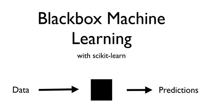
# #So why Bayesians?
# * Probabilistic Programming is a new paradigm.
# * Attributions: My friend Thomas Wiecki influenced a lot of my thinking on this.
# * I'm going to compare Blackbox Machine Learning with scikit-learn
#
# Attribution: http://www.sportsballshop.co.uk
# #Bayesian Rugby
# I came across the following blog post on http://danielweitzenfeld.github.io/passtheroc/blog/2014/10/28/bayes-premier-league/
#
#
#
# * Based on the work of [Baio and Blangiardo](http://www.statistica.it/gianluca/Research/BaioBlangiardo.pdf)
#
# * In this talk, I'm going to reproduce the first model described in the paper using pymc.
# * Since I am a rugby fan I decide to apply the results of the paper Bayesian Football to the Six Nations.
#
# #So why Bayesians?
# * Probabilistic Programming is a new paradigm.
# * Attributions: My friend Thomas Wiecki influenced a lot of my thinking on this.
# * I'm going to compare Blackbox Machine Learning with scikit-learn
#  #
# * Source: Olivier Grisel's talk on ML
#
# # Limitations of Machine learning
# * A big limitation of Machine Learning is that most of the models are black boxes.
#
#
#
#
# * Source: Olivier Grisel's talk on ML
#
# # Limitations of Machine learning
# * A big limitation of Machine Learning is that most of the models are black boxes.
#
#
#  #
# Source: Olivier Grisel's talk on ML
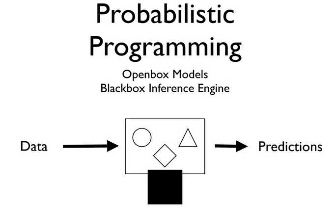
# # Probabilistic Programming - what's the big deal?
# * We are able to use data and our prior beliefs to generate a model.
# * Generating a model is extremely powerful
# * We can tell a story, which appeals to our understanding of stories.
#
# In[48]:
import os
import math
import warnings
import numpy as np
import pandas as pd
import matplotlib.pyplot as plt
import pymc # I know folks are switching to "as pm" but I'm just not there yet
get_ipython().run_line_magic('matplotlib', 'inline')
# # Six Nations Rugby
# * Rugby is a physical sport popular worldwide.
# * Six Nations consists of Italy, Ireland, Scotland, England, France and Wales
# * Game consists of scoring tries (similar to touch downs) or kicking the goal.
# * Average player is something like 100kg and 1.82m tall.
# * Paul O'Connell the Irish captain is Height: 6' 6" (1.98 m) Weight: 243 lbs (110 kg)
#
# #They compete for this!
# * Significant this year because the World Cup occurs in 2015.
#
#
# Source: Olivier Grisel's talk on ML
# # Probabilistic Programming - what's the big deal?
# * We are able to use data and our prior beliefs to generate a model.
# * Generating a model is extremely powerful
# * We can tell a story, which appeals to our understanding of stories.
#
# In[48]:
import os
import math
import warnings
import numpy as np
import pandas as pd
import matplotlib.pyplot as plt
import pymc # I know folks are switching to "as pm" but I'm just not there yet
get_ipython().run_line_magic('matplotlib', 'inline')
# # Six Nations Rugby
# * Rugby is a physical sport popular worldwide.
# * Six Nations consists of Italy, Ireland, Scotland, England, France and Wales
# * Game consists of scoring tries (similar to touch downs) or kicking the goal.
# * Average player is something like 100kg and 1.82m tall.
# * Paul O'Connell the Irish captain is Height: 6' 6" (1.98 m) Weight: 243 lbs (110 kg)
#
# #They compete for this!
# * Significant this year because the World Cup occurs in 2015.
#  # * Photo: Hostelrome
# ## Motivation
#
#
# * Your estimate of the strength of a team depends on your estimates of the other strengths
# * Ireland are a stronger team than Italy for example - but by how much?
# * Source for Results 2014 are Wikipedia.
# * I handcrafted these results
# * Small data
#
# * Photo: Hostelrome
# ## Motivation
#
#
# * Your estimate of the strength of a team depends on your estimates of the other strengths
# * Ireland are a stronger team than Italy for example - but by how much?
# * Source for Results 2014 are Wikipedia.
# * I handcrafted these results
# * Small data
#  # In[49]:
DATA_DIR = os.path.join(os.getcwd(), 'data/')
# In[50]:
#The results_2014 is a handcrafted results table from Wikipedia
data_file = DATA_DIR + 'results_2014.csv'
df = pd.read_csv(data_file, sep=',')
df.tail()
# In[51]:
teams = df.home_team.unique()
teams = pd.DataFrame(teams, columns=['team'])
teams['i'] = teams.index
teams.head()
# * Now we need to do some merging and munging
# In[52]:
df = pd.merge(df, teams, left_on='home_team', right_on='team', how='left')
df = df.rename(columns = {'i': 'i_home'}).drop('team', 1)
df = pd.merge(df, teams, left_on='away_team', right_on='team', how='left')
df = df.rename(columns = {'i': 'i_away'}).drop('team', 1)
df.head()
# In[53]:
observed_home_goals = df.home_score.values
observed_away_goals = df.away_score.values
home_team = df.i_home.values
away_team = df.i_away.values
num_teams = len(df.i_home.drop_duplicates())
num_games = len(home_team)
# Now we need to prepare the model for PyMC.
# In[54]:
g = df.groupby('i_away')
att_starting_points = np.log(g.away_score.mean())
g = df.groupby('i_home')
def_starting_points = -np.log(g.away_score.mean())
# # What do we want to infer?
# * We want to infer the latent paremeters (every team's strength) that are generating the data we observe (the scorelines).
# * Moreover, we know that the scorelines are a noisy measurement of team strength, so ideally, we want a model that makes it easy to quantify our uncertainty about the underlying strengths.
#
#
# # While my MCMC gently samples
# * Often we don't know what the Bayesian Model is explicitly, so we have to 'estimate' the Bayesian Model'
# * If we can't solve something, approximate it.
# * Markov-Chain Monte Carlo (MCMC) instead draws samples from the posterior.
# * Fortunately, this algorithm can be applied to almost any model.
#
# # What do we want?
# * We want to quantify our uncertainty
# * We want to also use this to generate a model
# * We want the answers as distributions *not* point estimates
# ## What assumptions do we know for our 'generative story'?
# * We know that the Six Nations in Rugby only has 6 teams.
# * We have data from last year!
# * We also know that in sports scoring is modelled as a Poisson distribution
#
# In[49]:
DATA_DIR = os.path.join(os.getcwd(), 'data/')
# In[50]:
#The results_2014 is a handcrafted results table from Wikipedia
data_file = DATA_DIR + 'results_2014.csv'
df = pd.read_csv(data_file, sep=',')
df.tail()
# In[51]:
teams = df.home_team.unique()
teams = pd.DataFrame(teams, columns=['team'])
teams['i'] = teams.index
teams.head()
# * Now we need to do some merging and munging
# In[52]:
df = pd.merge(df, teams, left_on='home_team', right_on='team', how='left')
df = df.rename(columns = {'i': 'i_home'}).drop('team', 1)
df = pd.merge(df, teams, left_on='away_team', right_on='team', how='left')
df = df.rename(columns = {'i': 'i_away'}).drop('team', 1)
df.head()
# In[53]:
observed_home_goals = df.home_score.values
observed_away_goals = df.away_score.values
home_team = df.i_home.values
away_team = df.i_away.values
num_teams = len(df.i_home.drop_duplicates())
num_games = len(home_team)
# Now we need to prepare the model for PyMC.
# In[54]:
g = df.groupby('i_away')
att_starting_points = np.log(g.away_score.mean())
g = df.groupby('i_home')
def_starting_points = -np.log(g.away_score.mean())
# # What do we want to infer?
# * We want to infer the latent paremeters (every team's strength) that are generating the data we observe (the scorelines).
# * Moreover, we know that the scorelines are a noisy measurement of team strength, so ideally, we want a model that makes it easy to quantify our uncertainty about the underlying strengths.
#
#
# # While my MCMC gently samples
# * Often we don't know what the Bayesian Model is explicitly, so we have to 'estimate' the Bayesian Model'
# * If we can't solve something, approximate it.
# * Markov-Chain Monte Carlo (MCMC) instead draws samples from the posterior.
# * Fortunately, this algorithm can be applied to almost any model.
#
# # What do we want?
# * We want to quantify our uncertainty
# * We want to also use this to generate a model
# * We want the answers as distributions *not* point estimates
# ## What assumptions do we know for our 'generative story'?
# * We know that the Six Nations in Rugby only has 6 teams.
# * We have data from last year!
# * We also know that in sports scoring is modelled as a Poisson distribution
#  # * Attribution: *Wikipedia*
# #The model.
#
# * Attribution: *Wikipedia*
# #The model.
# The league is made up by a total of T= 6 teams, playing each other once # in a season. We indicate the number of points scored by the home and the away team in the g-th game of the season (15 games) as $y_{g1}$ and $y_{g2}$ respectively.
#The vector of observed counts $\mathbb{y} = (y_{g1}, y_{g2})$ is modelled as independent Poisson: # $y_{gi}| \theta_{gj} \tilde\;\; Poisson(\theta_{gj})$ # where the theta parameters represent the scoring intensity in the g-th game for the team playing at home (j=1) and away (j=2), respectively.
# # # #We model these parameters according to a formulation that has been used widely in the statistical literature, assuming a log-linear random effect model: # $$log \theta_{g1} = home + att_{h(g)} + def_{a(g)} $$ # $$log \theta_{g2} = att_{a(g)} + def_{h(g)}$$ # the parameter home represents the advantage for the team hosting the game # and we assume that this effect is constant for all the teams and # throughout the season. # # # * Key assumption home effect is an advantage in Sports # * We know these things empirically from our 'domain specific' knowledge # * Bayesian Models allow you to incorporate *beliefs* or *knowledge* into your model! # # In addition, the scoring intensity is # determined jointly by the attack # and defense ability of the two teams involved, represented by the parameters att and def, respectively. # In line with the Bayesian approach, we have to specify some suitable prior distributions for all the # random parameters in our model. The variable $home$ # is modelled as a fixed effect, assuming a standard # flat prior distribution. We use the notation of describing the Normal distribution in terms of mean # and the precision. # $home \tilde\; Normal(0,0.0001)$
#Conversely, for each t = 1, ..., T, the team-specific effects are modelled as exchangeable from a common distribution: # $att_t \tilde\; Normal(\mu_{att}, \tau_{att})$ # and $def_t \tilde\; Normal(\mu_{def}, \tau_{def})$
#Note that they're breaking out team strength into attacking and defending strength. # A negative defense parameter will sap the mojo from the opposing team's attacking parameter.
# # #I made two tweaks to the model. It didn't make sense to me to have a $\mu_{att}$ when we're enforcing the sum-to-zero constraint by subtracting the mean anyway. So I eliminated $\mu_{att}$ and $\mu_{def}$
#Also because of the sum-to-zero constraint, # it seemed to me that we needed an intercept term in the log-linear model, capturing the average goals scored per game by the away team. # This we model with the following hyperprior. # $$intercept \tilde\; Normal(0, 0.001)$$
# # * The hyper-priors on the attack and defense parameters are also flat # * $\mu_att \tilde\; Normal(0,0.001)$ # * $\mu_def \tilde\; Normal(0,0.001)$ # * $\tau_att \tilde\; \Gamma(0.1,0.1)$ # * $\tau_def \tilde\; \Gamma(0.1,0.1)$ # ###Digression: Why the flat priors were picked (our hyperpriors are flat) # * There are lots of different ways of picking priors - see the literature # * I learned from this that it didn't make any difference to the results picking a uniform prior versus a flat prior # # Often it simply doesn't matter much what prior you use. # # # # # ###Definition: A prior distribution is non-informative if the prior is “flat” relative to the likelihood function. # # # * We are trying to have a reasonable model and let inference happen from the data set. # * ##Key takeaway - Often in Bayesian modelling it doesn't matter what your priors are. Let the data generate the story :) # In[55]: #hyperpriors - which apply to all teams home = pymc.Normal('home', 0, .0001, value=0) tau_att = pymc.Gamma('tau_att', .1, .1, value=10) tau_def = pymc.Gamma('tau_def', .1, .1, value=10) intercept = pymc.Normal('intercept', 0, .0001, value=0) #team-specific parameters atts_star = pymc.Normal("atts_star", mu=0, tau=tau_att, size=num_teams, value=att_starting_points.values) defs_star = pymc.Normal("defs_star", mu=0, tau=tau_def, size=num_teams, value=def_starting_points.values) # In[56]: # trick to code the sum to zero constraint @pymc.deterministic def atts(atts_star=atts_star): atts = atts_star.copy() atts = atts - np.mean(atts_star) return atts @pymc.deterministic def defs(defs_star=defs_star): defs = defs_star.copy() defs = defs - np.mean(defs_star) return defs @pymc.deterministic def home_theta(home_team=home_team, away_team=away_team, home=home, atts=atts, defs=defs, intercept=intercept): return np.exp(intercept + home + atts[home_team] + defs[away_team]) @pymc.deterministic def away_theta(home_team=home_team, away_team=away_team, home=home, atts=atts, defs=defs, intercept=intercept): return np.exp(intercept + atts[away_team] + defs[home_team]) # # Let us run the model! # * We specify the priors as Gamma distributions # # # In[57]: #likelihood of observed data home_points = pymc.Poisson('home_points', mu=home_theta, value=observed_home_goals, observed=True) away_points = pymc.Poisson('away_points', mu=away_theta, value=observed_away_goals, observed=True) #We need to approximate the Posterior by running a sampling algorithm mcmc = pymc.MCMC([home, intercept, tau_att, tau_def, home_theta, away_theta, atts_star, defs_star, atts, defs, home_points, away_points]) map_ = pymc.MAP( mcmc ) map_.fit() mcmc.sample(200000, 40000, 20) # #Diagnostics # Let's see if/how the model converged. # The home parameter looks good, and indicates that home field advantage amounts to goals per game at the intercept. # We can see that it converges just like the model for the Premier League in the other tutorial. # I wonder and this is left as a question if all field sports have models of this form that converge. # In[58]: pymc.Matplot.plot(home) # # * We can see in this analysis that home advantage gives about 0.55 points advantage. # * We also see not too much auto-correlation, so this looks quite good plot wise. # * We see here how *probabilistic programming* allows us to quantify our uncertainty about certain parameters. # # In[59]: pymc.Matplot.plot(atts) # We can plot all of the parameters, just to see. # In[60]: observed_season = DATA_DIR + 'table_2014.csv' df_observed = pd.read_csv(observed_season) df_observed.loc[df_observed.QR.isnull(), 'QR'] = '' df_avg = pd.DataFrame({'avg_att': atts.stats()['mean'], 'avg_def': defs.stats()['mean']}, index=teams.team.values) # In[61]: df_new = df_avg.merge(df_observed, left_index=True, right_on='team', how='left') #Bring in the new csv file df_results = pd.read_csv('df_avg_data_edited.csv', sep=';') # In[62]: df_results.tail() # In[63]: def fig3(): fig, ax = plt.subplots(figsize=(12,12)) for outcome in ['winners', 'wooden_spoon', 'triple_crown', 'NaN']: ax.plot(df_results.avg_att[df_results.QR == outcome], df_results.avg_def[df_results.QR == outcome], 'o', label=outcome) for label, x, y in zip(df_results.team.values, df_results.avg_att.values, df_results.avg_def.values): ax.annotate(label, xy=(x,y), xytext = (-5,5), textcoords = 'offset points') ax.set_title('Attack vs Defense avg effect: 13-14 Six Nations') ax.set_xlabel('Avg attack effect') ax.set_ylabel('Avg defense effect') ax.legend() # In[64]: fig3() # #Simulating a season # We would like to now simulate a season. Just to see what happens. # In[65]: def simulate_season(): """ Simulate a season once, using one random draw from the mcmc chain. """ num_samples = atts.trace().shape[0] draw = np.random.randint(0, num_samples) atts_draw = pd.DataFrame({'att': atts.trace()[draw, :],}) defs_draw = pd.DataFrame({'def': defs.trace()[draw, :],}) home_draw = home.trace()[draw] intercept_draw = intercept.trace()[draw] season = df.copy() season = pd.merge(season, atts_draw, left_on='i_home', right_index=True) season = pd.merge(season, defs_draw, left_on='i_home', right_index=True) season = season.rename(columns = {'att': 'att_home', 'def': 'def_home'}) season = pd.merge(season, atts_draw, left_on='i_away', right_index=True) season = pd.merge(season, defs_draw, left_on='i_away', right_index=True) season = season.rename(columns = {'att': 'att_away', 'def': 'def_away'}) season['home'] = home_draw season['intercept'] = intercept_draw season['home_theta'] = season.apply(lambda x: math.exp(x['intercept'] + x['home'] + x['att_home'] + x['def_away']), axis=1) season['away_theta'] = season.apply(lambda x: math.exp(x['intercept'] + x['att_away'] + x['def_home']), axis=1) season['home_goals'] = season.apply(lambda x: np.random.poisson(x['home_theta']), axis=1) season['away_goals'] = season.apply(lambda x: np.random.poisson(x['away_theta']), axis=1) season['home_outcome'] = season.apply(lambda x: 'win' if x['home_goals'] > x['away_goals'] else 'loss' if x['home_goals'] < x['away_goals'] else 'draw', axis=1) season['away_outcome'] = season.apply(lambda x: 'win' if x['home_goals'] < x['away_goals'] else 'loss' if x['home_goals'] > x['away_goals'] else 'draw', axis=1) season = season.join(pd.get_dummies(season.home_outcome, prefix='home')) season = season.join(pd.get_dummies(season.away_outcome, prefix='away')) return season def create_season_table(season): """ Using a season dataframe output by simulate_season(), create a summary dataframe with wins, losses, goals for, etc. """ g = season.groupby('i_home') home = pd.DataFrame({'home_goals': g.home_goals.sum(), 'home_goals_against': g.away_goals.sum(), 'home_wins': g.home_win.sum(), 'home_losses': g.home_loss.sum() }) g = season.groupby('i_away') away = pd.DataFrame({'away_goals': g.away_goals.sum(), 'away_goals_against': g.home_goals.sum(), 'away_wins': g.away_win.sum(), 'away_losses': g.away_loss.sum() }) df = home.join(away) df['wins'] = df.home_wins + df.away_wins df['losses'] = df.home_losses + df.away_losses df['points'] = df.wins * 2 df['gf'] = df.home_goals + df.away_goals df['ga'] = df.home_goals_against + df.away_goals_against df['gd'] = df.gf - df.ga df = pd.merge(teams, df, left_on='i', right_index=True) df = df.sort_index(by='points', ascending=False) df = df.reset_index() df['position'] = df.index + 1 df['champion'] = (df.position == 1).astype(int) df['relegated'] = (df.position > 5).astype(int) return df def simulate_seasons(n=100): dfs = [] for i in range(n): s = simulate_season() t = create_season_table(s) t['iteration'] = i dfs.append(t) return pd.concat(dfs, ignore_index=True) # # Simulation # * We are going to simulate 1000 seasons # # In[66]: simuls = simulate_seasons(1000) # In[67]: def fig1(): figsize(9,9) ax = simuls.points[simuls.team == 'Ireland'].hist() median = simuls.points[simuls.team == 'Ireland'].median() ax.set_title('Ireland: 2015 points, 1000 simulations') ax.plot([median, median], ax.get_ylim()) plt.annotate('Median: %s' % median, xy=(median + 1, ax.get_ylim()[1]-10)) # In[68]: fig1() # * So what have we learned so far, we've got 1000 simulations of Ireland and their median points in the table is 8. # * In Rugby you get 2 points per win, and there are 5 games per year. So this model predicted that Ireland would win most of the time 4 games. # # In[69]: def fig2(): ax = simuls.gf[simuls.team == 'Ireland'].hist(figsize=(7,5)) median = simuls.gf[simuls.team == 'Ireland'].median() ax.set_title('Ireland: 2015 scores for, 1000 simulations') ax.plot([median, median], ax.get_ylim()) plt.annotate('Median: %s' % median, xy=(median + 1, ax.get_ylim()[1]-10)) # In[70]: fig2() # #What happened in reality? # * Well Ireland actually scored 119 points, so the model over predicted this! # * We call this 'shrinkage' in the literature. # * All models are wrong, but some are useful # # What are the predictions of the model? # * So let us look at the winning team on average. # * We do a simulation and we'll assign probability of 'winning' to the team # * We used the MCMC to do this. # # In[71]: g = simuls.groupby('team') df_champs = pd.DataFrame({'percent_champs': g.champion.mean()}) df_champs = df_champs.sort_index(by='percent_champs') df_champs = df_champs[df_champs.percent_champs > .05] df_champs = df_champs.reset_index() # In[72]: fig, ax = plt.subplots(figsize=(8,6)) ax.barh(df_champs.index.values, df_champs.percent_champs.values) for i, row in df_champs.iterrows(): label = "{0:.1f}%".format(100 * row['percent_champs']) ax.annotate(label, xy=(row['percent_champs'], i), xytext = (3, 10), textcoords = 'offset points') ax.set_ylabel('Team') ax.set_title('% of Simulated Seasons In Which Team Finished Winners') _= ax.set_yticks(df_champs.index + .5) _= ax.set_yticklabels(df_champs['team'].values) # Unfortunately it seems that in most of the Universes England come top of the Six Nations. And as an Irish man this is firm proof that I put Mathematical rigour before patriotism :) # This is a reasonable result, and I hope it proved a nice example of Bayesian models in Rugby Analytics. # # What actually happened # We need to investigate like 'scientists' what actually happened. # # In[73]: pd.read_csv('data/results_2015.csv', sep='\t', header=0, names =['Rank','Team','Games','Wins','Draws', 'Losses','Points_For','Points_Against','Points']) # ##Ireland won the Six Nations! # * The model incorrectly predicted that England would come out on top. # * Ireland actually won by points difference of 6 points. # * It really came down to the wire! # In[74]: from IPython.display import Image Image(filename='onedoesnotsimply.jpg') # * One of the powers of Probabilistic Programming is that we can model 'latent' variables. # * In Quantitative Finance we could model the 'fear' of investors. While we can't measure this directly. # * In our Rugby Prediction model we are trying to infer the 'strength' of the team. Whereas in reality we can only measure the 'score' of the team. # # Bayes' formula allows us to then infer backwards: given the observable data (e.g. the stock price), what is the probability of the latent construct (e.g. investor fear)? # # Attribution: Thomas Wiecki at Quantopian influenced me on this. # # # What are the advantages of PyMC3? # What are the computational remarks? # Where is my table of contents? # Where is Bayes formula? # #Stochastic volatility model # One elegant example of how Probabilistic Programming can infer # unobservable quantities of the stock market is the stochastic volatility model. Volatility is an important concept of quantitative finance as it relates to risk. When I studied Financial Mathematics I was always confused about 'volatility' - since you can't measure it. # # If we can't measure something, the next best thing we can do is to try and model # it. One way to do this is in a probabilistic framework is the concept of stochastic # volatility: If we assume that returns are normally distributed, the volatility would be captured # as the standard deviation of the normal distribution. Thus, the standard deviation gives rise to stochastic volatility. Intuitively we would assume that the standard deviation is high during times of market turmoil like the 2008 crash. # # # So the trivial thing to do would be to look at the rolling standard deviation of returns. But this is unsatisfying for multiple reasons: # # * it often lags behind volatility, # * is a rather unstable measure, # * strongly dependent on the window size with no principled way of choosing it. # # In fact a lot of 'business processes' we encounter as Data Scientists can't be measured directly. We can only 'model' how likely a person is to churn from our service for example. # We can't infer exactly. # # # # # Introducing PyMC3 # * PyMC3 is a complete rewrite # * Uses Theano and all of its computational coolness rather than Fortran. # * The API is cleaner, but I found it difficult to use since I know PyMC2 better # * The example I'll show first is a FinTech example for Stochastic Volatility # * Attribution: The PyMC3 Development team. # # PyMC3 - continued # * Probabilistic Programming framework written in Python. # * Allows for construction of probabilistic models using intuitive syntax. # * Features advanced MCMC samplers. # * Fast: Just-in-time compiled by Theano. # * Extensible: easily incorporates custom MCMC algorithms and unusual probability distributions. # * Authors: John Salvatier, Chris Fonnesbeck, Thomas Wiecki # * Upcoming beta release! # # Why Theano? # # * Numpy broadcasting and advanced indexing # * Linear algebra operators # * Computation optimization and dynamic C compilation # # Other reasons # * Theano compiles computations down to C, making computations faster, especially larger models # # * Theano: automatic differentiation, automatic likelihood optimization and simple GPU integration. # # * Automatic differentiation is a different way to computationally work out derivatives unlike say Symbolic or Numeric Differentiation # # Other other reasons # (From John Salvatier the main author of PyMC3) # * Bayesian inference is a powerful and flexible way to learn from data, that is easy to understand. # Unfortunately larger problems are often computationally intractable. Markov Chain Monte Carlo sampling techniques help, but are still computationally limited. New gradient-based methods like the No U-Turn Sampler (NUTS) dramatically increase performance on hard problems. # # # # PyMC3 Sales Pitch :) # * From John Salvatier too # * PyMC 3 provides a easy and concise way to specify models and provides powerful yet easy to use samplers like NUTS. This enables users easily fit large and complex models with thousands of parameters. PyMC 3 is a complete rewrite of PyMC 2 based on Theano. PyMC expands its powerful NumPy-like syntax, and is now easier to extend and automatically optimized by Theano. # # Alternatives to PyMC3 # * [Frequentist and Bayesianism](http://arxiv.org/abs/1411.5018) - An article by Jake Vander Plas discusses emcee, PyStan and PyMC2 and compares them # * JAGS/BUGS are also alternatives # * All are non-Pythonic and are in fact domain specific languages # * There are challenges getting your data into and out of these # In[75]: import numpy as np import pymc3 as pm3 from pymc3.distributions.timeseries import GaussianRandomWalk from scipy.sparse import csc_matrix from scipy import optimize # Asset prices have time-varying volatility (variance of day over day returns). In some periods, returns are highly variable, while in others very stable. Stochastic volatility models model this with a latent volatility variable, modeled as a stochastic process. The following model is similar to the one described in the No-U-Turn Sampler paper, Hoffman (2011) p21. # * $\sigma \;\; \tilde \;\;Exponential(50)$ # # * $\mu \;\;\tilde \;\; Exponential(.1)$ # # * $s_i\;\; \tilde \;\; Normal(s_{i−1},\sigma−2)$ # # * $\log(\frac{y_i}{yi−1})\;\;\tilde \;\;t(\nu ,0,\exp(−2s_{i}))$ # # # Here, y is the daily return series and s is the latent log volatility process. # # # # Build the Model # In[116]: def fig4(): n = 400 returns = np.genfromtxt("data/S&P500.csv")[-n:] returns[:5] np.array([-0.00637 , -0.004045, -0.02547 , 0.005102, -0.047733]) plt.plot(returns) # In[77]: fig4() # * So so far we plotted our returns from the S and P 500. # Specifying the model in pymc3 mirrors its statistical specification. # # However, it is easier to sample the scale of the log volatility process innovations, σ, on a log scale, so we create it using TransformedVar and use logtransform. # # TransformedVar creates one variable in the transformed space and one in the normal space. The one in the transformed space (here log(σ)) is the one over which sampling will occur, and the one in the normal space is the one to use throughout the rest of the model. # # It takes a variable name, a distribution and a transformation to use. # # One of the strengths of the PyMC3 API is that it allows you to write statistics quite naturally. # # Personally it appeals to Data Developers like myself who are from a Mathematics Background. # # # In[78]: model = pm3.Model() with model: n = 400 returns = np.genfromtxt("data/S&P500.csv")[-n:] sigma, log_sigma = model.TransformedVar('sigma', pm3.Exponential.dist(1./.02, testval=.1), pm3.logtransform) nu = pm3.Exponential('nu', 1./10) s = GaussianRandomWalk('s', sigma**-2, shape=n) r = pm3.T('r', nu, lam=pm3.exp(-2*s), observed=returns) # # Fit the model # * Now that we have built the model and you can see the Syntax already. # * We need to fit the model. # # For this model, the full maximum a posteriori (MAP) point is degenerate and has infinite density. However, if we fix log_sigma and $\nu$ it is no longer degenerate, so we find the MAP with respect to the volatility process, 's', keeping log_sigma and $\nu$ constant at their default values. # # We use L-BFGS because it is more efficient for high dimensional functions (s has n elements). # # ### Key Tip: The usage of clever scaling parameters to avoid degeneracy is an art of Bayesian Statistics # In[79]: with model: start = pm3.find_MAP(vars=[s], fmin=optimize.fmin_l_bfgs_b) # We do a short initial run to get near the right area, then start again using a new Hessian at the new starting point to get faster sampling due to better scaling. # We do a short run since this is an interactive example. # In[80]: with model: step = pm3.NUTS(scaling=start) start2 = pm3.sample(500, step, progressbar=True)[-1] # Start next run at the last sampled position. step = pm3.NUTS(scaling=start2) trace = pm3.sample(2000, step, start=start2, progressbar=True) figsize(12,6) pm3.traceplot(trace, model.vars[:-1]); # * Looking at the returns over time and overlaying the estimated standard deviation we can see how the model tracks the volatility over time. # # * This is exactly the sort of insight we expected. # # * [PyMC3 Docs](http://pymc-devs.github.io/pymc3/stochastic_volatility/) # In[81]: plot(returns) plot(np.exp(trace[s][::10].T), 'r', alpha=.03); sd = np.exp(trace[s].T) plot(-np.exp(trace[s][::10].T), 'r', alpha=.03); xlabel('time') ylabel('returns') # # Rugby Analytics in PyMC3 # * This is a ported version of PyMC2 code that I already showed. # * Thanks to John Salvatier and Abraham Flaxman on Stackoverflow. # * Grateful to live in an age of open source and Stackoverflow # In[82]: get_ipython().system('date') import numpy as np import pandas as pd try: from StringIO import StringIO except ImportError: from io import StringIO get_ipython().run_line_magic('matplotlib', 'inline') import pymc3 as pm3, theano.tensor as tt # In[83]: data_csv = StringIO("""home_team,away_team,home_score,away_score Wales,Italy,23,15 France,England,26,24 Ireland,Scotland,28,6 Ireland,Wales,26,3 Scotland,England,0,20 France,Italy,30,10 Wales,France,27,6 Italy,Scotland,20,21 England,Ireland,13,10 Ireland,Italy,46,7 Scotland,France,17,19 England,Wales,29,18 Italy,England,11,52 Wales,Scotland,51,3 France,Ireland,20,22""") # * We do the same munging and cleaning as in PyMC2 # In[84]: df = pd.read_csv(data_csv) teams = df.home_team.unique() teams = pd.DataFrame(teams, columns=['team']) teams['i'] = teams.index df = pd.merge(df, teams, left_on='home_team', right_on='team', how='left') df = df.rename(columns = {'i': 'i_home'}).drop('team', 1) df = pd.merge(df, teams, left_on='away_team', right_on='team', how='left') df = df.rename(columns = {'i': 'i_away'}).drop('team', 1) observed_home_goals = df.home_score.values observed_away_goals = df.away_score.values home_team = df.i_home.values away_team = df.i_away.values num_teams = len(df.i_home.drop_duplicates()) num_games = len(home_team) g = df.groupby('i_away') att_starting_points = np.log(g.away_score.mean()) g = df.groupby('i_home') def_starting_points = -np.log(g.away_score.mean()) # * We will see now one of the major differences between PyMC2 and PyMC3 # * PyMC3 has more samplers. # * Also PyMC2 has the initial values specified in the model # * PyMC3 has the intitial values included when you fit the model. # In[85]: model = pm3.Model() with pm3.Model() as model: # global model parameters home = pm3.Normal('home', 0, .0001) tau_att = pm3.Gamma('tau_att', .1, .1) tau_def = pm3.Gamma('tau_def', .1, .1) intercept = pm3.Normal('intercept', 0, .0001) # team-specific model parameters atts_star = pm3.Normal("atts_star", mu =0, tau =tau_att, shape=num_teams) defs_star = pm3.Normal("defs_star", mu =0, tau =tau_def, shape=num_teams) atts = pm3.Deterministic('atts', atts_star - tt.mean(atts_star)) defs = pm3.Deterministic('defs', defs_star - tt.mean(defs_star)) home_theta = tt.exp(intercept + home + atts[away_team] + defs[home_team]) away_theta = tt.exp(intercept + atts[away_team] + defs[home_team]) # likelihood of observed data home_points = pm3.Poisson('home_points', mu=home_theta, observed=observed_home_goals) away_points = pm3.Poisson('away_points', mu=away_theta, observed=observed_away_goals) # * We specified the model and the likelihood function # * Now we need to fit our model using the Maximum A Posteriori algorithm to decide where to start out No U Turn Sampler # * All this runs on a Theano graph under the hood # * Very clever from a Computational Engineering point of view # * **Remark** The NUTS sampler is new from Gelman and triggered the rewrite # In[86]: with model: start = pm3.find_MAP() step = pm3.NUTS(state=start) trace = pm3.sample(2000, step, start=start, progressbar=True) pm3.traceplot(trace) # In[87]: pm3.forestplot(trace, vars=['tau_att', 'tau_def']); # In[88]: pm3.plots.summary(trace) # #Conclusion - Six Nations model # * 'All models are wrong, some are useful' # * Model correctly predicts that Ireland would win 4 games # * Model incorrectly predicted that England would come out on top # * In reality it was very close # * Recommendation: Don't use this model to bet on the Six Nations next years # The big difference, as I see it, between PyMC2 and 3 model building is that the whole business of initial values in PyMC2 is not included in model building in PyMC3. # It is pushed off into the model fitting portion of the code. # # A financial example # * We are going to use a Financial Example from Quantopian. - Thomas Wiecki produced this # * [Value at Risk](https://en.wikipedia.org/wiki/Value_at_risk) is a standard financial measure in risk. # * The underlying message will be to look at the distributional assumptions in our models. # * Bayesian Statistics makes these very explicit # # Why does this matter? # * A lot of models have naive assumptions like 'the underlying phenomenoa is a Gaussian distribution' # * Those of us who deal with ecommerce data or commodity data or whatever know this just isn't true # * I want to show the power of this framework in Fin Tech :) # # As we know: We want to approximate our Posterior with MCMC Sampling # In[89]: def plot_want_get(): from scipy import stats fig = plt.figure(figsize=(14, 6)) ax1 = fig.add_subplot(121, title='What we want', ylim=(0, .5), xlabel='', ylabel='') ax1.plot(np.linspace(-4, 4, 100), stats.norm.pdf(np.linspace(-3, 3, 100)), lw=4.) ax2 = fig.add_subplot(122, title='What we get')#, xlim=(-4, 4), ylim=(0, 1800), xlabel='', ylabel='\# of samples') sns.distplot(np.random.randn(50000), ax=ax2, kde=False, norm_hist=True); ax2.set_xlim((-4, 4)); ax2.set_ylim((0, .5)); # In[90]: plot_want_get() # # MCMC allows us to approximate an integral # * This is the basic idea behind simulation methods like Monte Carlo # * There are other samplers which work better for integrals with discontinuities etc # * We could teach an entire 3 day workshop on all this cool stuff :) # # # We want to model our returns - specify our Priors :) # # In[91]: import theano.tensor as T x = np.linspace(-.3, .3, 500) plt.plot(x, T.exp(pm3.Normal.dist(mu=0, sd=.1).logp(x)).eval()) plt.title(u'Prior: mu ~ Normal(0, $.1^2$)'); plt.xlabel('mu'); plt.ylabel('Probability Density'); plt.xlim((-.3, .3)); # In[92]: x = np.linspace(-.1, .5, 500) plt.plot(x, T.exp(pm3.HalfNormal.dist(sd=.1).logp(x)).eval()) plt.title(u'Prior: sigma ~ HalfNormal($.1^2$)'); plt.xlabel('sigma'); plt.ylabel('Probability Density'); # # Let us recap. # * We have specified our priors, in terms of $\mu$ and $\sigma$. # * We now need to specify our Bayesian Sharpe Ratio # * The Sharpe ratio is a common metric used to measure financial performance. # * This could be any classical metric in your field. # # Bayesian Sharpe Ratio # * $\mu \;\; \tilde \;\; Normal(0, .1^{2})$ <- Prior # * $\sigma \;\; \tilde \;\; HalfNormal(.1^{2})$ <- Prior # * Returns $\; \tilde \;\; Normal(\mu, \sigma^{2})$ <- Observed # * Sharpe ratio $= \frac{\mu}{\sigma}$ # # # #
# Attribution: Quantopian blog
# # Not a bad idea to show the data :)
# In[93]:
print(data_0.head())
# In[94]:
with pm3.Model() as model:
# Priors on Random Variables
mean_return = pm3.Normal('mean return', mu=0, sd=.1)
volatility = pm3.HalfNormal('volatility', sd=.1)
# Model returns as Normal
obs = pm3.Normal('returns',
mu=mean_return,
sd=volatility,
observed=data_0)
#There are 252 trading days in a year hence the 252 below
sharpe = pm3.Deterministic('sharpe ratio',
mean_return / volatility * np.sqrt(252))
# In[95]:
with model:
# Instantiate MCMC sampler - in fact a No-U turn sampler
step = pm3.NUTS()
# Draw 1000 samples from the posterior
trace = pm3.sample(1000, step)
# # Now that we need to analyse our Posterior.
# * Let us do some exploratory data analysis on our Posterior to see what it looks like
# In[96]:
sns.distplot(results_normal[0]['mean returns'], hist=False, label='etrade')
sns.distplot(results_normal[1]['mean returns'], hist=False, label='IB')
plt.title('Posterior of the mean'); plt.xlabel('mean returns')
# In[97]:
sns.distplot(results_normal[0]['volatility'], hist=False, label='etrade')
sns.distplot(results_normal[1]['volatility'], hist=False, label='IB')
plt.title('Posterior of the volatility')
plt.xlabel('volatility')
# In[98]:
sns.distplot(results_normal[0]['sharpe'], hist=False, label='etrade')
sns.distplot(results_normal[1]['sharpe'], hist=False, label='IB')
plt.title('Bayesian Sharpe ratio'); plt.xlabel('Sharpe ratio');
# In[99]:
print('P(Sharpe ratio IB > 0) = %.2f%%' % \
(np.mean(results_normal[1]['sharpe'] > 0) * 100))
# In[100]:
print('P(Sharpe ratio IB > Sharpe ratio etrade) = %.2f%%' % \
(np.mean(results_normal[1]['sharpe'] > results_normal[0][0]['sharpe']) * 100))
# # Value at Risk with uncertainty.
# * We want to now compute our Value at Risk with Uncertainty
# * This shows the power of the Probabilistic Programming approach
#
# In[101]:
results_normal[0]
# In[102]:
import scipy.stats as stats
ppc_etrade = post_pred(var_cov_var_normal, results_normal[0], 1e6, .05, samples=800)
ppc_ib = post_pred(var_cov_var_normal, results_normal[1], 1e6, .05, samples=800)
sns.distplot(ppc_etrade, label='etrade', norm_hist=True, hist=False, color='b')
sns.distplot(ppc_ib, label='IB', norm_hist=True, hist=False, color='g')
plt.title('VaR'); plt.legend(loc=0); plt.xlabel('5% daily Value at Risk (VaR) with \$1MM capital (in \$)');
plt.ylabel('Probability density'); plt.xticks(rotation=15);
# # Interim summary
# * Bayesian stats allows us to reformulate common risk metrics, use priors and quantify uncertainty.
# * IB strategy seems better in almost every regard. Is it though?
# # So far, let's add confidence
# In[103]:
sns.distplot(results_normal[0]['sharpe'], hist=False, label='etrade')
sns.distplot(results_normal[1]['sharpe'], hist=False, label='IB')
plt.title('Bayesian Sharpe ratio'); plt.xlabel('Sharpe ratio');
plt.axvline(data_0.mean() / data_0.std() * np.sqrt(252), color='b');
plt.axvline(data_1.mean() / data_1.std() * np.sqrt(252), color='g');
# In[104]:
x = np.linspace(-.03, .03, 500)
ppc_dist_normal = post_pred(eval_normal, results_normal[1], x=x)
ppc_dist_t = post_pred(eval_t, results_t[1], x=x)
# # How good is our model?
# * Remember Box said "All models are wrong some are useful!"
# * How useful is our model?
# In[105]:
sns.distplot(data_1, label='data IB', kde=False, norm_hist=True, color='.5')
for p in ppc_dist_normal:
plt.plot(x, p, c='r', alpha=.1)
plt.plot(x, p, c='r', alpha=.5, label='Normal model')
plt.xlabel('Daily returns')
plt.legend();
# #Can it be improved? Yes!
# * Identical model as before, but instead, use a heavy-tailed T distribution:
# * $returns\;\tilde \;\; T(\nu,\mu,\sigma^{2})$
#
# In[106]:
figsize(12, 12)
sns.distplot(data_1, label='data IB', kde=False, norm_hist=True, color='.5')
for p in ppc_dist_t:
plt.plot(x, p, c='y', alpha=.1)
plt.plot(x, p, c='y', alpha=.5, label='T model')
plt.xlabel('Daily returns')
plt.legend();
# # Volatility
# In[107]:
sns.distplot(results_normal[1]['annual volatility'], hist=False, label='normal')
sns.distplot(results_t[1]['annual volatility'], hist=False, label='T')
plt.xlim((0, 0.2))
plt.xlabel('Posterior of annual volatility')
plt.ylabel('Probability Density');
# # We need to compare posteriors
# In[108]:
sns.distplot(results_normal[1]['mean returns'], hist=False, color='r', label='normal model')
sns.distplot(results_t[1]['mean returns'], hist=False, color='y', label='T model')
plt.xlabel('Posterior of the mean returns'); plt.ylabel('Probability Density');
# # Bayesian T-sharpe ratio
# In[109]:
sns.distplot(results_normal[1]['sharpe'], hist=False, color='r', label='normal model')
sns.distplot(results_t[1]['sharpe'], hist=False, color='y', label='T model')
plt.xlabel('Bayesian Sharpe ratio'); plt.ylabel('Probability Density');
# # The robustness of the T-distribution is the strength of this model
# In[110]:
sim_data = list(np.random.randn(75)*.01)
sim_data.append(-.2)
sns.distplot(sim_data, label='data', kde=False, norm_hist=True, color='.5'); sns.distplot(sim_data, label='Normal', fit=stats.norm, kde=False, hist=False, fit_kws={'color': 'r', 'label': 'Normal'}); sns.distplot(sim_data, fit=stats.t, kde=False, hist=False, fit_kws={'color': 'y', 'label': 'T'})
plt.xlabel('Daily returns'); plt.legend();
# # Estimating tail risk using VaR
# In[111]:
ppc_normal = post_pred(var_cov_var_normal, results_normal[1], 1e6, .05, samples=800)
ppc_t = post_pred(var_cov_var_t, results_t[1], 1e6, .05, samples=800)
sns.distplot(ppc_normal, label='Normal', norm_hist=True, hist=False, color='r')
sns.distplot(ppc_t, label='T', norm_hist=True, hist=False, color='y')
plt.legend(loc=0); plt.xlabel('5% daily Value at Risk (VaR) with \$1MM capital (in \$)');
plt.ylabel('Probability density'); plt.xticks(rotation=15);
# # Comparing the Bayesian T-Sharpe Ratios
# In[112]:
sns.distplot(results_t[0]['sharpe'], hist=False, label='etrade')
sns.distplot(results_t[1]['sharpe'], hist=False, label='IB')
plt.xlabel('Bayesian Sharpe ratio'); plt.ylabel('Probability Density');
# In[113]:
print('P(Sharpe ratio IB > Sharpe ratio etrade) = %.2f%%' % \
(np.mean(results_t[1]['sharpe'] > results_t[0]['sharpe']) * 100))
# # Conclusion: Probabilistic Programming
# * **Probabilistic Programming** allows us to construct **complex models** in code and **automatically** estimate them.
# * **Bayesian statistics** provides us with **uncertainty quantification** -- measure orthogonal sources of **risk**.
# * **PyMC3** puts **advanced samplers** at your fingertips.
# * **PyMC2** is less powerful than **PyMC3**
#
# # Take home point
# * Bayesian Models by forcing you to specify your priors. Allow you to make better decisions under situations of uncertainty.
# * As Data Scientists we are always dealing with this.
# ##Want to learn more?
# * [Thomas Wiecki Blog on all things Bayesian](https://twiecki.github.io)
# * Twitter: [@springcoil](https://twitter.com/springcoil)
# * [Probabilistic Programming for Hackers](http://camdavidsonpilon.github.io/Probabilistic-Programming-and-Bayesian-Methods-for-Hackers/) -- IPython Notebook book on Bayesian stats using PyMC2
#
# * [Doing Bayesian Data Analysis](http://www.indiana.edu/~kruschke/DoingBayesianDataAnalysis/) -- Great book by Kruschke.
# * [Get PyMC3 alpha](https://github.com/pymc-devs/pymc/tree/pymc3)
# * [Zalando Example](http://dataconomy.com/how-zalando-used-bayesian-statistics-to-save-loads-of-money/)
# In[114]:
from IPython.display import Image
Image(filename='the-most-interesting-man-in-the-world-meme-generator-i-don-t-give-many-talks-but-when-i-do-i-do-q-a-e38222 copy.jpg')
# In[115]:
#Format from https://github.com/ellisonbg/talk-2013-scipy
from IPython.display import display, HTML
s = """
"""
display(HTML(s))