#!/usr/bin/env python
# coding: utf-8
# # Performing Quantum Measurements in QuTiP
#
# * EuroSciPy 2019
# * Simon Cross
# ### Outline
#
# * Why this weird quantum mechanics anyway?
# * Simulating a simple classical system.
# * What is a classical bit?
# * What is a qubit?
# * Measuring a qubit.
# * Simulating a simple quantum experiment in QuTiP.
# ### Meta goals
#
# * Use QuTiP to try things out.
# * Try understand what we're doing!
# # Imports: Our tools
# In[1]:
get_ipython().run_line_magic('matplotlib', 'inline')
from collections import namedtuple
import matplotlib.pyplot as plt
import numpy as np
import qutip
from qutip import Qobj, Bloch, basis, ket, tensor
# In[2]:
qutip.about()
# Define LaTeX commands:
# * $\newcommand{\ket}[1]{\left|{#1}\right\rangle}$ $\ket{0}$
# * $\newcommand{\bra}[1]{\left\langle{#1}\right|}$ $\bra{1}$
# * $\newcommand{\abs}[1]{\lvert{#1}\rvert}$ $\abs{x}$
# # The Stern-Gerlach Experiment
#
# Why this weird quantum mechanics anyway?
# ### Apparatus
#
# 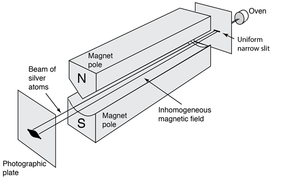 #
# Great drawing from: http://hyperphysics.phy-astr.gsu.edu/hbase/spin.html
# See also:
#
# * https://plato.stanford.edu/entries/physics-experiment/app5.html.
# * https://en.wikipedia.org/wiki/Stern%E2%80%93Gerlach_experiment#History
#
# for more on the history of the Stern-Gerlach experiment.
# Why did they decide to do this?
#
# It had become generally accepted that atoms could behave as tiny magnets.
#
# In the classical model of the atom, electrons orbit the nucleus. A charge orbiting in a circle generates a magnetic field -- so atoms should act like tiny magnets and be deflected by an inhomogenous magnetic field.
#
# Stern had the idea that this deflection would help better measure and understand the magnetic moment of the atoms & Gerlach brought the experimental expertise.
# \begin{align}
# F_z & = \mu_z \frac{\partial B}{\partial z} \\
# & = ( \hat{\mu} \cdot \hat{z} ) |\mu| \frac{\partial B}{\partial z} \\
# & \propto \hat{\mu} \cdot \hat{z}
# \end{align}
# Here $\hat \mu$ is the magnetic moment (strength and direction of the atom's magnetic field) and $\hat z$ is the direction in which the magnetic field varies (and which the measurement is made in).
#
# The assumptions that the magnitude of the the atoms magnetic moment $\abs{\mu}$ and the inhomogeneity of the magnetic field are constant allow us to make the last statement that $F_z$ is proportional to the dot product of $\hat \mu$ and $\hat z$.
#
# Now for fun, let's display the $\hat \mu$ and $\hat z$ vectors using QuTiP's `Bloch` class. For now consider this class just a handy way to plot vectors -- we will be learning more about what it is later on.
# In[3]:
z = np.array([0, 0, 1])
mu = np.array([0, 1, 1]) / np.sqrt(2)
bloch = Bloch()
bloch.zlabel=("z", "")
bloch.add_vectors([z, mu])
bloch.show()
# # Let's simulate the Stern-Gerlach in Python!
#
# Simulating a simple classical system.
# In[4]:
# Simulation of expected results in the classical case
Direction = namedtuple("Direction", ["theta", "phi"])
def random_direction():
""" Generate a random direction. """
# See http://mathworld.wolfram.com/SpherePointPicking.html
r = 0
while r == 0:
x, y, z = np.random.normal(0, 1, 3)
r = np.sqrt(x**2 + y**2 + z**2)
phi = np.arctan2(y, x)
theta = np.arccos(z / r)
return Direction(theta=theta, phi=phi)
# In[5]:
def classical_state(d):
""" Prepare a spin state given a direction. """
x = np.sin(d.theta) * np.cos(d.phi)
y = np.sin(d.theta) * np.sin(d.phi)
z = np.cos(d.theta)
return np.array([x, y, z])
# In[6]:
classical_up = np.array([0, 0, 1])
def classical_spin(c):
""" Measure the z-component of the spin. """
return classical_up.dot(c)
# In[7]:
def classical_stern_gerlach(n):
""" Simulate the Stern-Gerlach experiment """
directions = [random_direction() for _ in range(n)]
atoms = [classical_state(d) for d in directions]
spins = [classical_spin(c) for c in atoms]
return atoms, spins
# In[8]:
def plot_classical_results(atoms, spins):
fig = plt.figure(figsize=(18.0, 8.0))
fig.suptitle("Stern-Gerlach Experiment: Classical Outcome", fontsize="xx-large")
ax1 = plt.subplot(1, 2, 1, projection='3d')
ax2 = plt.subplot(1, 2, 2)
b = Bloch(fig=fig, axes=ax1)
b.vector_width = 1
b.vector_color = ["#ff{:x}0ff".format(i, i) for i in range(10)]
b.zlabel = ["$z$", ""]
b.add_vectors(atoms)
b.render(fig=fig, axes=ax1)
ax2.hist(spins)
ax2.set_xlabel("Z-component of spin")
ax2.set_ylabel("# of atoms")
# In[9]:
atoms, spins = classical_stern_gerlach(1000)
plot_classical_results(atoms, spins)
# # The actual results
#
#
#
# Great drawing from: http://hyperphysics.phy-astr.gsu.edu/hbase/spin.html
# See also:
#
# * https://plato.stanford.edu/entries/physics-experiment/app5.html.
# * https://en.wikipedia.org/wiki/Stern%E2%80%93Gerlach_experiment#History
#
# for more on the history of the Stern-Gerlach experiment.
# Why did they decide to do this?
#
# It had become generally accepted that atoms could behave as tiny magnets.
#
# In the classical model of the atom, electrons orbit the nucleus. A charge orbiting in a circle generates a magnetic field -- so atoms should act like tiny magnets and be deflected by an inhomogenous magnetic field.
#
# Stern had the idea that this deflection would help better measure and understand the magnetic moment of the atoms & Gerlach brought the experimental expertise.
# \begin{align}
# F_z & = \mu_z \frac{\partial B}{\partial z} \\
# & = ( \hat{\mu} \cdot \hat{z} ) |\mu| \frac{\partial B}{\partial z} \\
# & \propto \hat{\mu} \cdot \hat{z}
# \end{align}
# Here $\hat \mu$ is the magnetic moment (strength and direction of the atom's magnetic field) and $\hat z$ is the direction in which the magnetic field varies (and which the measurement is made in).
#
# The assumptions that the magnitude of the the atoms magnetic moment $\abs{\mu}$ and the inhomogeneity of the magnetic field are constant allow us to make the last statement that $F_z$ is proportional to the dot product of $\hat \mu$ and $\hat z$.
#
# Now for fun, let's display the $\hat \mu$ and $\hat z$ vectors using QuTiP's `Bloch` class. For now consider this class just a handy way to plot vectors -- we will be learning more about what it is later on.
# In[3]:
z = np.array([0, 0, 1])
mu = np.array([0, 1, 1]) / np.sqrt(2)
bloch = Bloch()
bloch.zlabel=("z", "")
bloch.add_vectors([z, mu])
bloch.show()
# # Let's simulate the Stern-Gerlach in Python!
#
# Simulating a simple classical system.
# In[4]:
# Simulation of expected results in the classical case
Direction = namedtuple("Direction", ["theta", "phi"])
def random_direction():
""" Generate a random direction. """
# See http://mathworld.wolfram.com/SpherePointPicking.html
r = 0
while r == 0:
x, y, z = np.random.normal(0, 1, 3)
r = np.sqrt(x**2 + y**2 + z**2)
phi = np.arctan2(y, x)
theta = np.arccos(z / r)
return Direction(theta=theta, phi=phi)
# In[5]:
def classical_state(d):
""" Prepare a spin state given a direction. """
x = np.sin(d.theta) * np.cos(d.phi)
y = np.sin(d.theta) * np.sin(d.phi)
z = np.cos(d.theta)
return np.array([x, y, z])
# In[6]:
classical_up = np.array([0, 0, 1])
def classical_spin(c):
""" Measure the z-component of the spin. """
return classical_up.dot(c)
# In[7]:
def classical_stern_gerlach(n):
""" Simulate the Stern-Gerlach experiment """
directions = [random_direction() for _ in range(n)]
atoms = [classical_state(d) for d in directions]
spins = [classical_spin(c) for c in atoms]
return atoms, spins
# In[8]:
def plot_classical_results(atoms, spins):
fig = plt.figure(figsize=(18.0, 8.0))
fig.suptitle("Stern-Gerlach Experiment: Classical Outcome", fontsize="xx-large")
ax1 = plt.subplot(1, 2, 1, projection='3d')
ax2 = plt.subplot(1, 2, 2)
b = Bloch(fig=fig, axes=ax1)
b.vector_width = 1
b.vector_color = ["#ff{:x}0ff".format(i, i) for i in range(10)]
b.zlabel = ["$z$", ""]
b.add_vectors(atoms)
b.render(fig=fig, axes=ax1)
ax2.hist(spins)
ax2.set_xlabel("Z-component of spin")
ax2.set_ylabel("# of atoms")
# In[9]:
atoms, spins = classical_stern_gerlach(1000)
plot_classical_results(atoms, spins)
# # The actual results
#
# 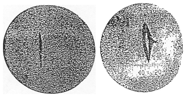 # In[10]:
def plot_real_vs_actual(spins):
fig = plt.figure(figsize=(18.0, 8.0))
fig.suptitle("Stern-Gerlach Experiment: Real vs Actual", fontsize="xx-large")
ax1 = plt.subplot(1, 2, 1)
ax2 = plt.subplot(1, 2, 2)
ax1.hist([np.random.choice([1, -1]) for _ in spins])
ax1.set_xlabel("Z-component of spin")
ax1.set_ylabel("# of atoms")
ax2.hist(spins)
ax2.set_xlabel("Z-component of spin")
ax2.set_ylabel("# of atoms")
# In[11]:
plot_real_vs_actual(spins)
# # Uh-oh.
#
# This really is a system with two outcomes.
# # If we align all the spins perpendicular to the z-axis:
#
# * Our classical simulator would show no force on any of the atoms.
# * The actual result would be the same as for the random spin case.
# # If we align all the spins with the z-axis:
#
# * Our classical simulator would show always 1.
# * The actual result would match that of the classical simulator.
# ## It's like tossing a biased coin.
# # Classical bit
#
# Something we're familiar with.
# ### Classical bit
#
# A *classical bit* (bit) is classical system with *two states* and *two outcomes*.
#
# * States: `0` and `1`
# * Outcomes: `0` and `1`
# ### Classical bit
#
# A *classical bit* (bit) is classical system with *two states* and *two outcomes*.
#
# * We can label these two states `0` and `1`.
# * Measuring state `0` produces an outcome which we will also label `0`.
# * Measuring state `1` produces an outcome which we will also label `1`.
# * These are the only two states.
# * Measuring the same state always produces the same outcome.
#
# The state is like a Python object. Measurement is an operation that acts on the state and returns an outcome.
#
# Bit is a portmanteau of *binary digit*.
#
# Examples:
#
# * A coin can lie on a surface in two different ways. We measure it by looking at it. We call the outcomes `heads` and `tails`.
# * A digital signal can have one of two different voltages. We measure it by measuring the voltage. We call the outcomes `high` and `low` (or `1` and `0`).
#
# With two bits there are four outcomes. With three bits there are eight outcomes. With `n` bits there are `2^n` outcomes.
#
# We need `n` bits to represent `n` bits.
# In[12]:
class ClassicalBit:
def __init__(self, outcome):
self.outcome = outcome
b0 = heads = ClassicalBit(outcome=0)
b1 = tails = ClassicalBit(outcome=1)
def measure_cbit(cbit):
return cbit.outcome
print("State:\n", b0)
print("Outcome:", measure_cbit(b0))
# # Quantum bit
#
# Putting the puzzle pieces together.
# ### Quantum bit
#
# A *quantum bit* (qubit) is quantum system with two *basis states* and *two outcomes*.
#
# * Basis states: `|0>` and `|1>`
# * Outcomes: `0` and `1`
#
# *Basis* means "we will construct more states from these later".
# ### Quantum Bit
#
# A *quantum bit* (qubit) is quantum system with two two *basis states* and two outcomes.
#
# * We can label these two basis states `|0>` and `|1>`.
# * Measuring state `|0>` produces an outcome which we will label `0`.
# * Measuring state `|1>` produces an outcome which we will label `1`.
# * There are other states called *superpositions* which we label `a|0> + b|1>`.
# * `a` and `b` are complex numbers.
# * Measuring a state produces outcome `0` with probability `|a|^2` and outcome `1` with probability `|b|^2`.
#
# Qubit is a portmanteau of *quantum bit* (it's portmanatees all the way down).
#
# Examples:
#
# * A coin can lie on a surface in two different ways. We measure it by looking at it. We call the outcomes `heads` and `tails`.
# * A digital signal can have one of two different volates. We measure it by measuring the voltage. We call the outcomes `high` and `low` (or `1` and `0`).
#
# With two qubits there are four outcomes. With three qubits there are eight outcomes. With `n` qubits there are `2^n` outcomes.
#
# We `2^n` (minus 1) complex numbers to represent `n` qubits.
# In[13]:
b0 = ket("0") # |0>
b1 = ket("1") # |1>
print("State:\n", b1)
# In[14]:
def measure_qbit(qbit):
if qbit == ket("0"):
return 0
if qbit == ket("1"):
return 1
raise NotImplementedError("No clue yet. :)")
print("Outcome:", measure_qbit(b1))
# # What about the "in between" states?
#
# The tricky part. :)
# # We want probabilistic outcomes
#
# Let's try something simple for the other states:
#
# * $a \ket{0} + b \ket{1}$
# * Probability of outcome $0$: $a$
# * Probability of outcome $1$: $b$
# We need:
#
# * $a + b = 1$
# * $1 >= a >= 0$
# * $1 >= b >= 0$
# In[15]:
def plot_real_a_b():
fig = plt.figure(figsize=(18.0, 8.0))
fig.suptitle("Probabilities: Real $a$ and $b$", fontsize="xx-large")
ax = plt.subplot(1, 1, 1)
ax.plot([0, 1], [1, 0])
ax.set_xlabel("$a$")
ax.set_xlim(-0.5, 1.5)
ax.set_ylabel("$b$")
ax.set_ylim(-0.5, 1.5)
# In[16]:
plot_real_a_b()
# # Hmm. That didn't work.
#
# Let's try something slightly more complicated:
#
# * $a \ket{0} + b \ket{1}$
# * $a, b \in \mathbb{C}$
# * Probability of outcome $0$: $\abs{a}^2$
# * Probability of outcome $1$: $\abs{b}^2$
#
# In[10]:
def plot_real_vs_actual(spins):
fig = plt.figure(figsize=(18.0, 8.0))
fig.suptitle("Stern-Gerlach Experiment: Real vs Actual", fontsize="xx-large")
ax1 = plt.subplot(1, 2, 1)
ax2 = plt.subplot(1, 2, 2)
ax1.hist([np.random.choice([1, -1]) for _ in spins])
ax1.set_xlabel("Z-component of spin")
ax1.set_ylabel("# of atoms")
ax2.hist(spins)
ax2.set_xlabel("Z-component of spin")
ax2.set_ylabel("# of atoms")
# In[11]:
plot_real_vs_actual(spins)
# # Uh-oh.
#
# This really is a system with two outcomes.
# # If we align all the spins perpendicular to the z-axis:
#
# * Our classical simulator would show no force on any of the atoms.
# * The actual result would be the same as for the random spin case.
# # If we align all the spins with the z-axis:
#
# * Our classical simulator would show always 1.
# * The actual result would match that of the classical simulator.
# ## It's like tossing a biased coin.
# # Classical bit
#
# Something we're familiar with.
# ### Classical bit
#
# A *classical bit* (bit) is classical system with *two states* and *two outcomes*.
#
# * States: `0` and `1`
# * Outcomes: `0` and `1`
# ### Classical bit
#
# A *classical bit* (bit) is classical system with *two states* and *two outcomes*.
#
# * We can label these two states `0` and `1`.
# * Measuring state `0` produces an outcome which we will also label `0`.
# * Measuring state `1` produces an outcome which we will also label `1`.
# * These are the only two states.
# * Measuring the same state always produces the same outcome.
#
# The state is like a Python object. Measurement is an operation that acts on the state and returns an outcome.
#
# Bit is a portmanteau of *binary digit*.
#
# Examples:
#
# * A coin can lie on a surface in two different ways. We measure it by looking at it. We call the outcomes `heads` and `tails`.
# * A digital signal can have one of two different voltages. We measure it by measuring the voltage. We call the outcomes `high` and `low` (or `1` and `0`).
#
# With two bits there are four outcomes. With three bits there are eight outcomes. With `n` bits there are `2^n` outcomes.
#
# We need `n` bits to represent `n` bits.
# In[12]:
class ClassicalBit:
def __init__(self, outcome):
self.outcome = outcome
b0 = heads = ClassicalBit(outcome=0)
b1 = tails = ClassicalBit(outcome=1)
def measure_cbit(cbit):
return cbit.outcome
print("State:\n", b0)
print("Outcome:", measure_cbit(b0))
# # Quantum bit
#
# Putting the puzzle pieces together.
# ### Quantum bit
#
# A *quantum bit* (qubit) is quantum system with two *basis states* and *two outcomes*.
#
# * Basis states: `|0>` and `|1>`
# * Outcomes: `0` and `1`
#
# *Basis* means "we will construct more states from these later".
# ### Quantum Bit
#
# A *quantum bit* (qubit) is quantum system with two two *basis states* and two outcomes.
#
# * We can label these two basis states `|0>` and `|1>`.
# * Measuring state `|0>` produces an outcome which we will label `0`.
# * Measuring state `|1>` produces an outcome which we will label `1`.
# * There are other states called *superpositions* which we label `a|0> + b|1>`.
# * `a` and `b` are complex numbers.
# * Measuring a state produces outcome `0` with probability `|a|^2` and outcome `1` with probability `|b|^2`.
#
# Qubit is a portmanteau of *quantum bit* (it's portmanatees all the way down).
#
# Examples:
#
# * A coin can lie on a surface in two different ways. We measure it by looking at it. We call the outcomes `heads` and `tails`.
# * A digital signal can have one of two different volates. We measure it by measuring the voltage. We call the outcomes `high` and `low` (or `1` and `0`).
#
# With two qubits there are four outcomes. With three qubits there are eight outcomes. With `n` qubits there are `2^n` outcomes.
#
# We `2^n` (minus 1) complex numbers to represent `n` qubits.
# In[13]:
b0 = ket("0") # |0>
b1 = ket("1") # |1>
print("State:\n", b1)
# In[14]:
def measure_qbit(qbit):
if qbit == ket("0"):
return 0
if qbit == ket("1"):
return 1
raise NotImplementedError("No clue yet. :)")
print("Outcome:", measure_qbit(b1))
# # What about the "in between" states?
#
# The tricky part. :)
# # We want probabilistic outcomes
#
# Let's try something simple for the other states:
#
# * $a \ket{0} + b \ket{1}$
# * Probability of outcome $0$: $a$
# * Probability of outcome $1$: $b$
# We need:
#
# * $a + b = 1$
# * $1 >= a >= 0$
# * $1 >= b >= 0$
# In[15]:
def plot_real_a_b():
fig = plt.figure(figsize=(18.0, 8.0))
fig.suptitle("Probabilities: Real $a$ and $b$", fontsize="xx-large")
ax = plt.subplot(1, 1, 1)
ax.plot([0, 1], [1, 0])
ax.set_xlabel("$a$")
ax.set_xlim(-0.5, 1.5)
ax.set_ylabel("$b$")
ax.set_ylim(-0.5, 1.5)
# In[16]:
plot_real_a_b()
# # Hmm. That didn't work.
#
# Let's try something slightly more complicated:
#
# * $a \ket{0} + b \ket{1}$
# * $a, b \in \mathbb{C}$
# * Probability of outcome $0$: $\abs{a}^2$
# * Probability of outcome $1$: $\abs{b}^2$
#  #
#  # # Complex numbers summary
#
# * $a = x + y \cdot j$
# * Length: $\sqrt{x^2 + y^2}$
# * Angle ($\theta$): $arctan(y / x)$
# * Python:
# * Length: `np.abs(a)`
# * Angle ($\theta$): `np.angle(a)`
# # Complex numbers in terms of length and angle
#
# * $a = m \cdot cos(t) + m \cdot sin(t) \cdot j$
# * $a = m \cdot e ^ {t \cdot j}$
# * Length: $m$
# * Angle: $t$
# # Global phase
#
# * 4 real parameters, minus one from $\abs{a}^2 + \abs{b}^2 = 1$
# * Still one too many.
# * Let's remove one!
# * Declare that only the relative angles of $a$ and $b$ are important.
# This means we can rotate the two vectors on the complex plane as long as we don't change the angle between them. Note that this doesn't change the magnitude of a or b (and thus doesn't change the probabilities).
# # The qubit states
#
# * General state: `a|0> + b|1>`
# * where $a$ and $b$ are complex numbers
# * $\abs{a}^2 + \abs{b}^2 = 1$
# * global phase is irrelevant:
# * $a = a \cdot e^{t \cdot j}, b = b \cdot e^{t \cdot j}$
# * Outcome:
# * `0` with probability $\abs{a}^2$
# * `1` with probability $\abs{b}^2$
# ### Bloch sphere
#
# This leaves only two real numbers:
#
# * The relative magnitudes of `|a|` and `|b|`.
# * The relative angle between `a` and `b`.
#
# Both of these form circles -- and the together the two circles form a sphere!
#
# Named after Felix Block (also the first director of CERN!)
# Wow, this looks a lot like a direction in space! Making progress!
# # How to sound smart at parties
#
# * SU(2) is isomorphic to SO(3)
# * `SU(2)` - the state space of qubits, aka the bloch sphere.
# * `SO(3)` - the space of directions in 3D, aka a sphere.
# * The state space of possible qubits is a sphere.
# # QuTiP has nice tools for visualising Bloch spheres
# In[17]:
b = Bloch()
b.show()
# In[18]:
b = Bloch()
up = ket("0")
down = ket("1")
b.add_states([up, down])
b.show()
# In[19]:
x = (up + down).unit()
y = (up + (0 + 1j) * down).unit()
z = up
b = Bloch()
b.add_states([x, y, z])
b.show()
# In[20]:
def plot_bloch(fig, ax, title, states, color_template):
""" Plot some states on the bloch sphere. """
b = Bloch(fig=fig, axes=ax)
ax.set_title(title, y=-0.01)
b.vector_width = 1
b.vector_color = [color_template.format(i * 10) for i in range(len(states))]
b.add_states(states)
b.render(fig=fig, axes=ax)
# In[21]:
def plot_multi_blochs(plots):
""" Plot multiple sets of states on bloch spheres. """
fig = plt.figure(figsize=(18.0, 8.0))
fig.suptitle("Bloch Sphere", fontsize="xx-large")
n = len(plots)
axes = [plt.subplot(1, n, i + 1, projection='3d') for i in range(n)]
for i, (title, states, color_template) in enumerate(plots):
plot_bloch(fig, axes[i], title, states, color_template)
# In[22]:
up = ket("0")
down = ket("1")
# magnitude_circle = [Qobj([[a], [np.sqrt(1 - a**2)]]) for a in np.linspace(0, 1, 20)]
magnitude_circle = [
(a * up + np.sqrt(1 - a**2) * down)
for a in np.linspace(0, 1, 20)
]
# angular_circle = [Qobj([[np.sqrt(0.5)], [np.sqrt(0.5) * np.e ** (1j * theta)]]) for theta in np.linspace(0, np.pi, 20)]
angular_circle = [
(np.sqrt(0.5) * up + np.sqrt(0.5) * down * np.e ** (1j * theta))
for theta in np.linspace(0, np.pi, 20)
]
# In[23]:
plot_multi_blochs([
["Changing relative magnitude", magnitude_circle, "#ff{:02x}ff"],
["Changing relative angle", angular_circle, "#{:02x}ffff"],
])
# # Measuring a general state
# In[24]:
def measure_qbit(qbit):
a = qbit.full()[0][0] # a
b = qbit.full()[1][0] # b
if np.random.random() <= np.abs(a) ** 2:
return 0
else:
return 1
# In[25]:
# |a|**2 + |b|**2 == 1
a = (1 + 0j) / np.sqrt(2)
b = (0 + 1j) / np.sqrt(2)
qbit = a * ket("0") + b * ket("1")
print("State:\n", qbit)
print("Outcome:", measure_qbit(qbit))
# In[26]:
qbit = (1 * ket("0")) + (1j * ket("1"))
qbit = qbit.unit()
print("State:\n", qbit)
print("Outcome:", measure_qbit(qbit))
# ### Other measures
#
# * Was there really anything special about $\ket{0}$ and $\ket{1}$?
# * No! :D
# * Except they pointed in opposite directions.
# * Can we make other measurements?
# * Yes!
# In[27]:
def component(qbit, direction):
component_op = direction.dag()
a = component_op * qbit
return a[0][0]
def measure_qbit(qbit, direction):
a = component(qbit, direction)
if np.random.random() <= np.abs(a) ** 2:
return 0
else:
return 1
# In[28]:
up, down = ket("0"), ket("1")
x, y, z = (up + down).unit(), (up + (0 + 1j) * down).unit(), up
print("State:\n", x)
print("Outcomes:", [measure_qbit(x, direction=up) for _ in range(10)])
# # Let's simulate the Stern-Gerlach with QuTiP!
#
# Simulating a simple ~~classical~~ quantum system.
# In[29]:
def quantum_state(d):
""" Prepare a spin state given a direction. """
return np.cos(d.theta / 2) * up + np.exp(1j * d.phi) * np.sin(d.theta / 2) * down
# In[30]:
up = ket('0')
def quantum_spin(q):
""" Measurement the z-component of the spin. """
a_up = (up.dag() * q).tr()
prob_up = np.abs(a_up) ** 2
return 1 if np.random.uniform(0, 1) <= prob_up else -1
# In[31]:
def quantum_stern_gerlach(n):
""" Simulate the Stern-Gerlach experiment """
directions = [random_direction() for _ in range(n)]
atoms = [quantum_state(d) for d in directions]
spins = [quantum_spin(q) for q in atoms]
return atoms, spins
# In[32]:
def plot_quantum_results(atoms, spins):
fig = plt.figure(figsize=(18.0, 8.0))
fig.suptitle("Stern-Gerlach Experiment: Quantum Outcome", fontsize="xx-large")
ax1 = plt.subplot(1, 2, 1, projection='3d')
ax2 = plt.subplot(1, 2, 2)
b = Bloch(fig=fig, axes=ax1)
b.vector_width = 1
b.vector_color = ["#{:x}0{:x}0ff".format(i, i) for i in range(10)]
b.add_states(atoms)
b.render(fig=fig, axes=ax1)
ax2.hist(spins)
ax2.set_xlabel("Z-component of spin")
ax2.set_ylabel("# of atoms")
# In[33]:
atoms, spins = quantum_stern_gerlach(1000)
plot_quantum_results(atoms, spins)
# # Further reading
#
# 1. QuTiP documentation [ https://qutip.org/ ]
#
# 2. Quantum Computing for the Determined by Michael Nielsen
# [ https://michaelnielsen.org/blog/quantum-computing-for-the-determined/ ]
#
# 3. Quantum Computing StackExchange
# [ https://quantumcomputing.stackexchange.com/ ]
#
# 4. History of the Stern-Gerlach experiment
# [ https://plato.stanford.edu/entries/physics-experiment/app5.html ]
#
# 5. Picking a random point on a sphere
# [ http://mathworld.wolfram.com/SpherePointPicking.html ]
# # The End
# # Complex numbers summary
#
# * $a = x + y \cdot j$
# * Length: $\sqrt{x^2 + y^2}$
# * Angle ($\theta$): $arctan(y / x)$
# * Python:
# * Length: `np.abs(a)`
# * Angle ($\theta$): `np.angle(a)`
# # Complex numbers in terms of length and angle
#
# * $a = m \cdot cos(t) + m \cdot sin(t) \cdot j$
# * $a = m \cdot e ^ {t \cdot j}$
# * Length: $m$
# * Angle: $t$
# # Global phase
#
# * 4 real parameters, minus one from $\abs{a}^2 + \abs{b}^2 = 1$
# * Still one too many.
# * Let's remove one!
# * Declare that only the relative angles of $a$ and $b$ are important.
# This means we can rotate the two vectors on the complex plane as long as we don't change the angle between them. Note that this doesn't change the magnitude of a or b (and thus doesn't change the probabilities).
# # The qubit states
#
# * General state: `a|0> + b|1>`
# * where $a$ and $b$ are complex numbers
# * $\abs{a}^2 + \abs{b}^2 = 1$
# * global phase is irrelevant:
# * $a = a \cdot e^{t \cdot j}, b = b \cdot e^{t \cdot j}$
# * Outcome:
# * `0` with probability $\abs{a}^2$
# * `1` with probability $\abs{b}^2$
# ### Bloch sphere
#
# This leaves only two real numbers:
#
# * The relative magnitudes of `|a|` and `|b|`.
# * The relative angle between `a` and `b`.
#
# Both of these form circles -- and the together the two circles form a sphere!
#
# Named after Felix Block (also the first director of CERN!)
# Wow, this looks a lot like a direction in space! Making progress!
# # How to sound smart at parties
#
# * SU(2) is isomorphic to SO(3)
# * `SU(2)` - the state space of qubits, aka the bloch sphere.
# * `SO(3)` - the space of directions in 3D, aka a sphere.
# * The state space of possible qubits is a sphere.
# # QuTiP has nice tools for visualising Bloch spheres
# In[17]:
b = Bloch()
b.show()
# In[18]:
b = Bloch()
up = ket("0")
down = ket("1")
b.add_states([up, down])
b.show()
# In[19]:
x = (up + down).unit()
y = (up + (0 + 1j) * down).unit()
z = up
b = Bloch()
b.add_states([x, y, z])
b.show()
# In[20]:
def plot_bloch(fig, ax, title, states, color_template):
""" Plot some states on the bloch sphere. """
b = Bloch(fig=fig, axes=ax)
ax.set_title(title, y=-0.01)
b.vector_width = 1
b.vector_color = [color_template.format(i * 10) for i in range(len(states))]
b.add_states(states)
b.render(fig=fig, axes=ax)
# In[21]:
def plot_multi_blochs(plots):
""" Plot multiple sets of states on bloch spheres. """
fig = plt.figure(figsize=(18.0, 8.0))
fig.suptitle("Bloch Sphere", fontsize="xx-large")
n = len(plots)
axes = [plt.subplot(1, n, i + 1, projection='3d') for i in range(n)]
for i, (title, states, color_template) in enumerate(plots):
plot_bloch(fig, axes[i], title, states, color_template)
# In[22]:
up = ket("0")
down = ket("1")
# magnitude_circle = [Qobj([[a], [np.sqrt(1 - a**2)]]) for a in np.linspace(0, 1, 20)]
magnitude_circle = [
(a * up + np.sqrt(1 - a**2) * down)
for a in np.linspace(0, 1, 20)
]
# angular_circle = [Qobj([[np.sqrt(0.5)], [np.sqrt(0.5) * np.e ** (1j * theta)]]) for theta in np.linspace(0, np.pi, 20)]
angular_circle = [
(np.sqrt(0.5) * up + np.sqrt(0.5) * down * np.e ** (1j * theta))
for theta in np.linspace(0, np.pi, 20)
]
# In[23]:
plot_multi_blochs([
["Changing relative magnitude", magnitude_circle, "#ff{:02x}ff"],
["Changing relative angle", angular_circle, "#{:02x}ffff"],
])
# # Measuring a general state
# In[24]:
def measure_qbit(qbit):
a = qbit.full()[0][0] # a
b = qbit.full()[1][0] # b
if np.random.random() <= np.abs(a) ** 2:
return 0
else:
return 1
# In[25]:
# |a|**2 + |b|**2 == 1
a = (1 + 0j) / np.sqrt(2)
b = (0 + 1j) / np.sqrt(2)
qbit = a * ket("0") + b * ket("1")
print("State:\n", qbit)
print("Outcome:", measure_qbit(qbit))
# In[26]:
qbit = (1 * ket("0")) + (1j * ket("1"))
qbit = qbit.unit()
print("State:\n", qbit)
print("Outcome:", measure_qbit(qbit))
# ### Other measures
#
# * Was there really anything special about $\ket{0}$ and $\ket{1}$?
# * No! :D
# * Except they pointed in opposite directions.
# * Can we make other measurements?
# * Yes!
# In[27]:
def component(qbit, direction):
component_op = direction.dag()
a = component_op * qbit
return a[0][0]
def measure_qbit(qbit, direction):
a = component(qbit, direction)
if np.random.random() <= np.abs(a) ** 2:
return 0
else:
return 1
# In[28]:
up, down = ket("0"), ket("1")
x, y, z = (up + down).unit(), (up + (0 + 1j) * down).unit(), up
print("State:\n", x)
print("Outcomes:", [measure_qbit(x, direction=up) for _ in range(10)])
# # Let's simulate the Stern-Gerlach with QuTiP!
#
# Simulating a simple ~~classical~~ quantum system.
# In[29]:
def quantum_state(d):
""" Prepare a spin state given a direction. """
return np.cos(d.theta / 2) * up + np.exp(1j * d.phi) * np.sin(d.theta / 2) * down
# In[30]:
up = ket('0')
def quantum_spin(q):
""" Measurement the z-component of the spin. """
a_up = (up.dag() * q).tr()
prob_up = np.abs(a_up) ** 2
return 1 if np.random.uniform(0, 1) <= prob_up else -1
# In[31]:
def quantum_stern_gerlach(n):
""" Simulate the Stern-Gerlach experiment """
directions = [random_direction() for _ in range(n)]
atoms = [quantum_state(d) for d in directions]
spins = [quantum_spin(q) for q in atoms]
return atoms, spins
# In[32]:
def plot_quantum_results(atoms, spins):
fig = plt.figure(figsize=(18.0, 8.0))
fig.suptitle("Stern-Gerlach Experiment: Quantum Outcome", fontsize="xx-large")
ax1 = plt.subplot(1, 2, 1, projection='3d')
ax2 = plt.subplot(1, 2, 2)
b = Bloch(fig=fig, axes=ax1)
b.vector_width = 1
b.vector_color = ["#{:x}0{:x}0ff".format(i, i) for i in range(10)]
b.add_states(atoms)
b.render(fig=fig, axes=ax1)
ax2.hist(spins)
ax2.set_xlabel("Z-component of spin")
ax2.set_ylabel("# of atoms")
# In[33]:
atoms, spins = quantum_stern_gerlach(1000)
plot_quantum_results(atoms, spins)
# # Further reading
#
# 1. QuTiP documentation [ https://qutip.org/ ]
#
# 2. Quantum Computing for the Determined by Michael Nielsen
# [ https://michaelnielsen.org/blog/quantum-computing-for-the-determined/ ]
#
# 3. Quantum Computing StackExchange
# [ https://quantumcomputing.stackexchange.com/ ]
#
# 4. History of the Stern-Gerlach experiment
# [ https://plato.stanford.edu/entries/physics-experiment/app5.html ]
#
# 5. Picking a random point on a sphere
# [ http://mathworld.wolfram.com/SpherePointPicking.html ]
# # The End