#!/usr/bin/env python # coding: utf-8 #
# # UFF logo # # # IC logo # #
# # Evolutionary Multi-Objective Optimization # # ## Luis Martí, [IC](http://www.ic.uff.br)/[UFF](http://www.uff.br) # # [http://lmarti.com](http://lmarti.com); [lmarti@ic.uff.br](mailto:lmarti@ic.uff.br) # # [Advanced Evolutionary Computation: Theory and Practice](http://lmarti.com/aec-2014) # This notebook is better viewed rendered as slides. You can convert it to slides and view them by: # - using [nbconvert](http://ipython.org/ipython-doc/1/interactive/nbconvert.html) with a command like: # ```bash # $ ipython nbconvert --to slides --post serve # ``` # - installing [Reveal.js - Jupyter/IPython Slideshow Extension](https://github.com/damianavila/live_reveal) # - using the online [IPython notebook slide viewer](https://slideviewer.herokuapp.com/) (some slides of the notebook might not be properly rendered). # # This and other related IPython notebooks can be found at the course github repository: # * [https://github.com/lmarti/evolutionary-computation-course](https://github.com/lmarti/evolutionary-computation-course) # # In this notebook # # * Present the basic concepts related to evolutionary multi-objective optimization algorithms. # * The Non-dominated Sorting Genetic Algorithm II (NSGA-II). # * Benchmark test problems. # * Experiment design and results comparison. # ## How can we handle multiple conflicting objectives? # # Even choosing a fruit implies dealing with conflicting objectives. # #
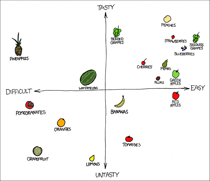
# taken from http://xkcd.com/388/
# # [Multi-objective optimization](http://en.wikipedia.org/wiki/Multi-objective_optimization) # # * Most -*if not all*- optimization problems involve more than one objective function to be optimized simultaneously. # * For example, you must optimize a given feature of an object while keeping under control the resources needed to elaborate that object. # * Sometimes those other objectives are converted to constraints or fixed to default values, but that does not means that they are there. # * Multi-objective optimization is also known as *multi-objective programming*, *vector optimization*, *multicriteria optimization*, *multiattribute optimization* or *Pareto optimization* (and probably by other names, depending on the field). # * Multi-objective optimization has been applied in [many fields of science](http://en.wikipedia.org/wiki/Multi-objective_optimization#Examples_of_multi-objective_optimization_applications), including engineering, economics and logistics (see the section on applications for detailed examples) where optimal decisions need to be taken in the presence of trade-offs between two or more conflicting objectives. # ## A Multi-objective Optimization Problem (MOP) # # $$ # \renewcommand{\vec}[1]{\mathbf{#1}} # \newcommand{\set}[1]{\mathcal{#1}} # \newcommand{\dom}{\preccurlyeq} # \left. # \begin{array}{rl} # \mathrm{minimize} & \vec{F}(\vec{x})=\langle f_1(\vec{x}),\ldots,f_M(\vec{x})\rangle\,,\\ # \mathrm{subject}\ \mathrm{to} & c_1(\vec{x}),\ldots,c_C(\vec{x})\le 0\,,\\ # & d_1(\vec{x}),\ldots,d_D(\vec{x})= 0\,,\\ # & \text{with}\ \vec{x}\in\set{D}\,, # \end{array}\right\} # $$ # # * $\mathcal{D}$ is known as the *decision set* or *search set*. # * functions $f_1(\mathbf{x}),\ldots,f_M(\mathbf{x})$ are the *objective functions*. If $M=1$ the problem reduces to a single-objective optimization problem. # * Image set, $\set{O}$, result of the projection of $\set{D}$ via $f_1(\vec{x}),\ldots,f_M(\vec{x})$ is called *objective set* ($\vec{F}:\set{D}\rightarrow\set{O}$). # * $c_1(\vec{x}),\ldots,c_C(\vec{x})\le 0$ and $d_1(\vec{x}),\ldots,d_D(\vec{x})= 0$ express the constraints imposed on the values of $\vec{x}$. # # *Note:* In case you are -still- wondering, a maximization problem can be posed as the minimization one: $\min\ -\vec{F}(\vec{x})$. # ## Example: A two variables and two objectives MOP # # ## MOP (optimal) solutions # # Usually, there is not a unique solution that minimizes all objective functions simultaneously, but, instead, a set of equally good *trade-off* solutions. # # * *Optimality* can be defined in terms of the [*Pareto dominance*](https://en.wikipedia.org/wiki/Pareto_efficiency) relation. That is, having $\vec{x},\vec{y}\in\set{D}$, $\vec{x}$ is said to dominate $\vec{y}$ (expressed as $\vec{x}\dom\vec{y}$) iff $\forall f_j$, $f_j(\vec{x})\leq f_j(\vec{y})$ and $\exists f_i$ such that $f_i(\vec{x})< f_i(\vec{y})$. # * Having the set $\set{A}$. $\set{A}^\ast$, the *non-dominated subset* of $\set{A}$, is defined as # # $$ # \set{A}^\ast=\left\{ \vec{x}\in\set{A} \left|\not\exists\vec{y}\in\set{A}:\vec{y}\dom\vec{x}\right.\right\}. # $$ # # * The *Pareto-optimal set*, $\set{D}^{\ast}$, is the solution of the problem. It is the subset of non-dominated elements of $\set{D}$. It is also known as the *efficient set*. # * It consists of solutions that cannot be improved in any of the objectives without degrading at least one of the other objectives. # * 
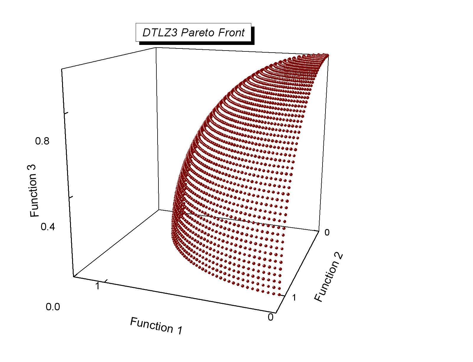
Its image in objective set is called the *Pareto-optimal front*, $\set{O}^\ast$. # * Evolutionary algorithms generally yield a set of non-dominated solutions, $\set{P}^\ast$, that approximates $\set{D}^{\ast}$. # # As usual, we need some initialization and configuration. # In[1]: import time, array, random, copy, math import numpy as np import pandas as pd # In[2]: import matplotlib.pyplot as plt get_ipython().run_line_magic('matplotlib', 'inline') get_ipython().run_line_magic('config', "InlineBackend.figure_format = 'retina'") plt.rc('text', usetex=True) plt.rc('font', family='serif') plt.rcParams['text.latex.preamble'] ='\\usepackage{libertine}\n\\usepackage[utf8]{inputenc}' import seaborn seaborn.set(style='whitegrid') seaborn.set_context('notebook') # In[3]: from deap import algorithms, base, benchmarks, tools, creator # Planting a constant seed to always have the same results (and avoid surprises in class). -*you should not do this in a real-world case!* # In[4]: random.seed(a=42) # # Visualizing the Pareto dominance relation # # * To start, lets have a visual example of the Pareto dominance relationship in action. # * In this notebook we will deal with two-objective problems in order to simplify visualization. # * Therefore, we can create: # In[5]: creator.create("FitnessMin", base.Fitness, weights=(-1.0,-1.0)) creator.create("Individual", array.array, typecode='d', fitness=creator.FitnessMin) # ## Let's use an illustrative MOP problem: Dent # # $$ # \begin{array}{rl} # \text{minimize} & f_1(\vec{x}),f_2(\vec{x}) \\ # \text{such that} & f_1(\vec{x}) = \frac{1}{2}\left( \sqrt{1 + (x_1 + x_2)^2} \sqrt{1 + (x_1 - x_2)^2} + x_1 -x_2\right) + d,\\ # & f_2(\vec{x}) = \frac{1}{2}\left( \sqrt{1 + (x_1 + x_2)^2} \sqrt{1 + (x_1 - x_2)^2} - x_1 -x_2\right) + d,\\ # \text{with}& d = \lambda e^{-\left(x_1-x_2\right)^2}\ (\text{generally }\lambda=0.85) \text{ and } \vec{x}\in \left[-1.5,1.5\right]^2. # \end{array} # $$ # Implementing the Dent problem # In[6]: def dent(individual, lbda = 0.85): """ Implements the test problem Dent Num. variables = 2; bounds in [-1.5, 1.5]; num. objetives = 2. @author Cesar Revelo """ d = lbda * math.exp(-(individual[0] - individual[1]) ** 2) f1 = 0.5 * (math.sqrt(1 + (individual[0] + individual[1]) ** 2) + \ math.sqrt(1 + (individual[0] - individual[1]) ** 2) + \ individual[0] - individual[1]) + d f2 = 0.5 * (math.sqrt(1 + (individual[0] + individual[1]) ** 2) + \ math.sqrt(1 + (individual[0] - individual[1]) ** 2) - \ individual[0] + individual[1]) + d return f1, f2 # Preparing a DEAP `toolbox` with Dent. # In[7]: toolbox = base.Toolbox() # In[8]: BOUND_LOW, BOUND_UP = -1.5, 1.5 NDIM = 2 # toolbox.register("evaluate", lambda ind: benchmarks.dtlz2(ind, 2)) toolbox.register("evaluate", dent) # Defining attributes, individuals and population. # In[9]: def uniform(low, up, size=None): try: return [random.uniform(a, b) for a, b in zip(low, up)] except TypeError: return [random.uniform(a, b) for a, b in zip([low] * size, [up] * size)] toolbox.register("attr_float", uniform, BOUND_LOW, BOUND_UP, NDIM) toolbox.register("individual", tools.initIterate, creator.Individual, toolbox.attr_float) toolbox.register("population", tools.initRepeat, list, toolbox.individual) # Creating an example population distributed as a mesh. # In[10]: num_samples = 50 limits = [np.arange(BOUND_LOW, BOUND_UP, (BOUND_UP - BOUND_LOW)/num_samples)] * NDIM sample_x = np.meshgrid(*limits) # In[11]: flat = [] for i in range(len(sample_x)): x_i = sample_x[i] flat.append(x_i.reshape(num_samples**NDIM)) # In[12]: example_pop = toolbox.population(n=num_samples**NDIM) # In[13]: for i, ind in enumerate(example_pop): for j in range(len(flat)): ind[j] = flat[j][i] # In[14]: fitnesses = toolbox.map(toolbox.evaluate, example_pop) for ind, fit in zip(example_pop, fitnesses): ind.fitness.values = fit # We also need `a_given_individual`. # In[15]: a_given_individual = toolbox.population(n=1)[0] a_given_individual[0] = 0.5 a_given_individual[1] = 0.5 # In[16]: a_given_individual.fitness.values = toolbox.evaluate(a_given_individual) # Implementing the Pareto dominance relation between two individulas. # In[17]: def pareto_dominance(ind1,ind2): 'Returns `True` if `ind1` dominates `ind2`.' extrictly_better = False for item1 in ind1.fitness.values: for item2 in ind2.fitness.values: if item1 > item2: return False if not extrictly_better and item1 < item2: extrictly_better = True return extrictly_better # *Note:* Bear in mind that DEAP comes with a Pareto dominance relation that probably is more efficient than this implementation. # ```python # def pareto_dominance(x,y): # return tools.emo.isDominated(x.fitness.values, y.fitness.values) # ``` # Lets compute the set of individuals that are `dominated` by `a_given_individual`, the ones that dominate it (its `dominators`) and the remaining ones. # In[18]: dominated = [ind for ind in example_pop if pareto_dominance(a_given_individual, ind)] dominators = [ind for ind in example_pop if pareto_dominance(ind, a_given_individual)] others = [ind for ind in example_pop if not ind in dominated and not ind in dominators] # In[19]: def plot_dent(): 'Plots the points in decision and objective spaces.' plt.figure(figsize=(10,5)) plt.subplot(1,2,1) for ind in dominators: plt.plot(ind[0], ind[1], 'r.') for ind in dominated: plt.plot(ind[0], ind[1], 'g.') for ind in others: plt.plot(ind[0], ind[1], 'k.', ms=3) plt.plot(a_given_individual[0], a_given_individual[1], 'bo', ms=6); plt.xlabel('$x_1$');plt.ylabel('$x_2$'); plt.title('Decision space'); plt.subplot(1,2,2) for ind in dominators: plt.plot(ind.fitness.values[0], ind.fitness.values[1], 'r.', alpha=0.7) for ind in dominated: plt.plot(ind.fitness.values[0], ind.fitness.values[1], 'g.', alpha=0.7) for ind in others: plt.plot(ind.fitness.values[0], ind.fitness.values[1], 'k.', alpha=0.7, ms=3) plt.plot(a_given_individual.fitness.values[0], a_given_individual.fitness.values[1], 'bo', ms=6); plt.xlabel('$f_1(\mathbf{x})$');plt.ylabel('$f_2(\mathbf{x})$'); plt.xlim((0.5,3.6));plt.ylim((0.5,3.6)); plt.title('Objective space'); plt.tight_layout() # Having `a_given_individual` (blue dot) we can now plot those that are dominated by it (in green), those that dominate it (in red) and those that are uncomparable. # In[20]: plot_dent() # Obtaining the nondominated front. # In[21]: non_dom = tools.sortNondominated(example_pop, k=len(example_pop), first_front_only=True)[0] # In[22]: plt.figure(figsize=(5,5)) for ind in example_pop: plt.plot(ind.fitness.values[0], ind.fitness.values[1], 'k.', ms=3, alpha=0.5) for ind in non_dom: plt.plot(ind.fitness.values[0], ind.fitness.values[1], 'bo', alpha=0.74, ms=5) plt.title('Pareto-optimal front') # # The Non-dominated Sorting Genetic Algorithm (NSGA-II) # # * NSGA-II algorithm is one of the pillars of the EMO field. # * Deb, K., Pratap, A., Agarwal, S., Meyarivan, T., *A fast and elitist multiobjective genetic algorithm: NSGA-II*, IEEE Transactions on Evolutionary Computation, vol.6, no.2, pp.182,197, Apr 2002 doi: [10.1109/4235.996017](http://dx.doi.org/10.1109/4235.996017). # * Fitness assignment relies on the Pareto dominance relation: # 1. Rank individuals according the dominance relations established between them. # 2. Individuals with the same domination rank are then compared using a local crowding distance. # ## NSGA-II fitness in detail # # * The first step consists in classifying the individuals in a series of categories $\mathcal{F}_1,\ldots,\mathcal{F}_L$. # * Each of these categories store individuals that are only dominated by the elements of the previous categories, # $$ # \begin{array}{rl} # \forall \vec{x}\in\set{F}_i: &\exists \vec{y}\in\set{F}_{i-1} \text{ such that } \vec{y}\dom\vec{x},\text{ and }\\ # &\not\exists\vec{z}\in \set{P}_t\setminus\left( \set{F}_1\cup\ldots\cup\set{F}_{i-1} # \right)\text{ that }\vec{z}\dom\vec{x}\,; # \end{array} # $$ # with $\mathcal{F}_1$ equal to $\mathcal{P}_t^\ast$, the set of non-dominated individuals of $\mathcal{P}_t$. # # * After all individuals are ranked a local crowding distance is assigned to them. # * The use of this distance primes individuals more isolated with respect to others. # ## Crowding distance # # The assignment process goes as follows, # # * for each category set $\set{F}_l$, having $f_l=|\set{F}_l|$, # * for each individual $\vec{x}_i\in\set{F}_l$, set $d_{i}=0$. # * for each objective function $m=1,\ldots,M$, # * $\vec{I}=\mathrm{sort}\left(\set{F}_l,m\right)$ (generate index vector). # * $d_{I_1}^{(l)}=d_{I_{f_l}}^{(l)}=\infty$. # * for $i=2,\ldots,f_l-1$, # * Update the remaining distances as, # $$ # d_i = d_i + \frac{f_m\left(\vec{x}_{I_{i+1}}\right)-f_m\left(\vec{x}_{I_{i+1}}\right)} # {f_m\left(\vec{x}_{I_{1}}\right)-f_m\left(\vec{x}_{I_{f_l}}\right)}\,. # $$ # # Here the $\mathrm{sort}\left(\set{F},m\right)$ function produces an ordered index vector $\vec{I}$ with respect to objective function $m$. # Sorting the population by rank and distance. # # * Having the individual ranks and their local distances they are sorted using the crowded comparison operator, stated as: # * An individual $\vec{x}_i$ _is better than_ $\vec{x}_j$ if: # * $\vec{x}_i$ has a better rank: $\vec{x}_i\in\set{F}_k$, $\vec{x}_j\in\set{F}_l$ and $kd_j$. # # **Now we have key element of the the non-dominated sorting GA.** # ## Implementing NSGA-II # # We will deal with [DTLZ3](http://www.tik.ee.ethz.ch/sop/download/supplementary/testproblems/dtlz3/), which is a more difficult test problem. # # * DTLZ problems can be configured to have as many objectives as desired, but as we want to visualize results we will stick to two objectives. # * DTLZ3 is a (more complex) version of [DTLZ2](http://www.tik.ee.ethz.ch/sop/download/supplementary/testproblems/dtlz2/). # * The Pareto-optimal front of DTLZ3 lies in the first [orthant](http://en.wikipedia.org/wiki/Orthant) of a unit (radius 1) hypersphere located at the coordinate origin ($\vec{0}$). # * It has many local optima that run parallel to the global optima and render the optimization process more complicated. # #
# from Coello Coello, Lamont and Van Veldhuizen (2007) Evolutionary Algorithms for Solving Multi-Objective Problems, Second Edition. Springer [Appendix E](http://www.cs.cinvestav.mx/~emoobook/apendix-e/apendix-e.html).
# New `toolbox` instance with the necessary components. # In[23]: toolbox = base.Toolbox() # Define problem domain as $\vec{x}\in\left[0,1\right]^{30}$ and a two-objective DTLZ3 instance. # In[24]: NDIM = 30 BOUND_LOW, BOUND_UP = 0.0, 1.0 toolbox.register("evaluate", lambda ind: benchmarks.dtlz3(ind, 2)) # Describing attributes, individuals and population and defining the selection, mating and mutation operators. # In[25]: toolbox.register("attr_float", uniform, BOUND_LOW, BOUND_UP, NDIM) toolbox.register("individual", tools.initIterate, creator.Individual, toolbox.attr_float) toolbox.register("population", tools.initRepeat, list, toolbox.individual) toolbox.register("mate", tools.cxSimulatedBinaryBounded, low=BOUND_LOW, up=BOUND_UP, eta=20.0) toolbox.register("mutate", tools.mutPolynomialBounded, low=BOUND_LOW, up=BOUND_UP, eta=20.0, indpb=1.0/NDIM) toolbox.register("select", tools.selNSGA2) # Let's also use the `toolbox` to store other configuration parameters of the algorithm. This will show itself usefull when performing massive experiments. # In[26]: toolbox.pop_size = 50 toolbox.max_gen = 1000 toolbox.mut_prob = 0.2 # ## A compact NSGA-II implementation # # Storing all the required information in the `toolbox` and using DEAP's `algorithms.eaMuPlusLambda` function allows us to create a very compact -albeit not a 100% exact copy of the original- implementation of NSGA-II. # In[27]: def run_ea(toolbox, stats=None, verbose=False): pop = toolbox.population(n=toolbox.pop_size) pop = toolbox.select(pop, len(pop)) return algorithms.eaMuPlusLambda(pop, toolbox, mu=toolbox.pop_size, lambda_=toolbox.pop_size, cxpb=1-toolbox.mut_prob, mutpb=toolbox.mut_prob, stats=stats, ngen=toolbox.max_gen, verbose=verbose) # ## Running the algorithm # We are now ready to run our NSGA-II. # In[28]: get_ipython().run_line_magic('time', 'res,_ = run_ea(toolbox)') # We can now get the Pareto fronts in the results (`res`). # In[29]: fronts = tools.emo.sortLogNondominated(res, len(res)) # ## Resulting Pareto fronts # In[30]: plot_colors = seaborn.color_palette("Set1", n_colors=10) fig, ax = plt.subplots(1, figsize=(4,4)) for i,inds in enumerate(fronts): par = [toolbox.evaluate(ind) for ind in inds] df = pd.DataFrame(par) df.plot(ax=ax, kind='scatter', label='Front ' + str(i+1), x=df.columns[0], y=df.columns[1], color=plot_colors[i]) plt.xlabel('$f_1(\mathbf{x})$');plt.ylabel('$f_2(\mathbf{x})$'); # * It is better to make an animated plot of the evolution as it takes place. # ## Animating the evolutionary process # We create a `stats` to store the individuals not only their objective function values. # In[31]: stats = tools.Statistics() stats.register("pop", copy.deepcopy) # In[32]: toolbox.max_gen = 1000 # we need more generations! # Re-run the algorithm to get the data necessary for plotting. # In[33]: get_ipython().run_line_magic('time', 'res, logbook = run_ea(toolbox, stats=stats)') # In[34]: from matplotlib import animation from IPython.display import HTML # In[35]: def animate(frame_index, logbook): 'Updates all plots to match frame _i_ of the animation.' ax.clear() fronts = tools.emo.sortLogNondominated(logbook.select('pop')[frame_index], len(logbook.select('pop')[frame_index])) for i,inds in enumerate(fronts): par = [toolbox.evaluate(ind) for ind in inds] df = pd.DataFrame(par) df.plot(ax=ax, kind='scatter', label='Front ' + str(i+1), x=df.columns[0], y=df.columns[1], alpha=0.47, color=plot_colors[i % len(plot_colors)]) ax.set_title('$t=$' + str(frame_index)) ax.set_xlabel('$f_1(\mathbf{x})$');ax.set_ylabel('$f_2(\mathbf{x})$') return [] # In[36]: fig = plt.figure(figsize=(4,4)) ax = fig.gca() anim = animation.FuncAnimation(fig, lambda i: animate(i, logbook), frames=len(logbook), interval=60, blit=True) plt.close() # In[37]: HTML(anim.to_html5_video()) # Here it is clearly visible how the algorithm "jumps" from one local-optimum to a better one as evolution takes place. # # MOP benchmark problem toolkits # # Each problem instance is meant to test the algorithms with regard with a given feature: local optima, convexity, discontinuity, bias, or a combination of them. # # * [*ZDT1-6*](http://www.tik.ee.ethz.ch/sop/download/supplementary/testproblems/): Two-objective problems with a fixed number of decision variables. # * E. Zitzler, K. Deb, and L. Thiele. Comparison of Multiobjective Evolutionary Algorithms: Empirical Results. Evolutionary Computation, 8(2):173-195, 2000. ([pdf](http://www.tik.ee.ethz.ch/sop/publicationListFiles/zdt2000a.pdf)) # * [*DTLZ1-7*](http://www.tik.ee.ethz.ch/sop/download/supplementary/testproblems/): $m$-objective problems with $n$ variables. # * K. Deb, L. Thiele, M. Laumanns and E. Zitzler. Scalable Multi-Objective Optimization Test Problems. CEC 2002, p. 825 - 830, IEEE Press, 2002. ([pdf](http://www.tik.ee.ethz.ch/sop/publicationListFiles/dtlz2002a.pdf)) # * [*CEC'09*](http://dces.essex.ac.uk/staff/zhang/moeacompetition09.htm): Two- and three- objective problems that very complex Pareto sets. # * Zhang, Q., Zhou, A., Zhao, S., & Suganthan, P. N. (2009). Multiobjective optimization test instances for the CEC 2009 special session and competition. In 2009 IEEE Congress on Evolutionary Computation (pp. 1–30). ([pdf](http://dces.essex.ac.uk/staff/zhang/MOEAcompetition/cec09testproblem0904.pdf.pdf)) # * [*WFG1-9*](http://www.wfg.csse.uwa.edu.au/publications.html#toolkit): $m$-objective problems with $n$ variables, very complex. # * Huband, S., Hingston, P., Barone, L., & While, L. (2006). A review of multiobjective test problems and a scalable test problem toolkit. IEEE Transactions on Evolutionary Computation, 10(5), 477–506. doi:10.1109/TEVC.2005.861417 # How does our NSGA-II behaves when faced with different benchmark problems? # In[38]: problem_instances = {'ZDT1': benchmarks.zdt1, 'ZDT2': benchmarks.zdt2, 'ZDT3': benchmarks.zdt3, 'ZDT4': benchmarks.zdt4, 'DTLZ1': lambda ind: benchmarks.dtlz1(ind,2), 'DTLZ2': lambda ind: benchmarks.dtlz2(ind,2), 'DTLZ3': lambda ind: benchmarks.dtlz3(ind,2), 'DTLZ4': lambda ind: benchmarks.dtlz4(ind,2, 100), 'DTLZ5': lambda ind: benchmarks.dtlz5(ind,2), 'DTLZ6': lambda ind: benchmarks.dtlz6(ind,2), 'DTLZ7': lambda ind: benchmarks.dtlz7(ind,2)} # In[39]: toolbox.max_gen = 1000 stats = tools.Statistics(lambda ind: ind.fitness.values) stats.register("obj_vals", np.copy) def run_problem(toolbox, problem): toolbox.register('evaluate', problem) return run_ea(toolbox, stats=stats) # Running NSGA-II solving all problems. Now it takes longer. # In[40]: get_ipython().run_line_magic('time', 'results = {problem: run_problem(toolbox, problem_instances[problem]) for problem in problem_instances}') # Creating this animation takes more programming effort. # In[41]: class MultiProblemAnimation: def init(self, fig, results): self.results = results self.axs = [fig.add_subplot(3,4,i+1) for i in range(len(results))] self.plots =[] for i, problem in enumerate(sorted(results)): (res, logbook) = self.results[problem] pop = pd.DataFrame(data=logbook.select('obj_vals')[0]) plot = self.axs[i].plot(pop[0], pop[1], 'b.', alpha=0.47)[0] self.plots.append(plot) fig.tight_layout() def animate(self, t): 'Updates all plots to match frame _i_ of the animation.' for i, problem in enumerate(sorted(results)): #self.axs[i].clear() (res, logbook) = self.results[problem] pop = pd.DataFrame(data=logbook.select('obj_vals')[t]) self.plots[i].set_data(pop[0], pop[1]) self.axs[i].set_title(problem + '; $t=' + str(t)+'$') self.axs[i].set_xlim((0, max(1,pop.max()[0]))) self.axs[i].set_ylim((0, max(1,pop.max()[1]))) return self.axs # In[42]: mpa = MultiProblemAnimation() # In[43]: fig = plt.figure(figsize=(14,6)) anim = animation.FuncAnimation(fig, mpa.animate, init_func=mpa.init(fig,results), frames=toolbox.max_gen, interval=60, blit=True) plt.close() # In[44]: HTML(anim.to_html5_video()) # * It is interesting how the algorithm deals with each problem: clearly some problems are harder than others. # * In some cases it "hits" the Pareto front and then slowly explores it. # # **Read more about this in the class materials.** # # Experiment design and reporting results # # * Watching an animation of an EMO algorithm solve a problem is certainly fun. # * It also allows us to understand many particularities of the problem being solved. # * But, as [Carlos Coello](http://delta.cs.cinvestav.mx/~ccoello/) would say, we are *not* in an art appreciation class. # * We should follow the key concepts provided by the [scientific method](http://en.wikipedia.org/wiki/Scientific_method). # * I urge you to study the [experimental design](http://en.wikipedia.org/wiki/Design_of_experiments) topic in depth as it is an essential knowledge. # # **Evolutionary algorithms are stochastic algorithms, therefore their results must be assessed by repeating experiments until you reach an statistically valid conclusion.** # ## An illustrative simple/sample experiment # # Let's make a relatively simple but very important experiment: # # * **Question**: In our NSGA-II applied to a two-objective DTLZ3 problem: Is it more important to have a big population and let the algorithm run for a few iterations or is better to have a small population and let the algorithm run for larger number of iterations. # * **Procedure**: We must perform an experiment testing different population sizes and maximum number of iterations while keeping the other parameters constant. # ### Notation # # As usual we need to establish some notation: # # * *Multi-objective problem* (or just *problem*): A multi-objective optimization problem, as defined above. # * *MOEA*: An evolutionary computation method used to solve multi-objective problems. # * *Experiment*: a combination of problem and MOEA and a set of values of their parameters. # * *Experiment run*: The result of running an experiment. # * We will use `toolbox` instances to define experiments. # We start by creating a `toolbox` that will contain the configuration that will be shared across all experiments. # In[45]: toolbox = base.Toolbox() # In[46]: BOUND_LOW, BOUND_UP = 0.0, 1.0 NDIM = 30 # the explanation of this... a few lines bellow def eval_helper(ind): return benchmarks.dtlz3(ind, 2) toolbox.register("evaluate", eval_helper) # In[47]: def uniform(low, up, size=None): try: return [random.uniform(a, b) for a, b in zip(low, up)] except TypeError: return [random.uniform(a, b) for a, b in zip([low] * size, [up] * size)] toolbox.register("attr_float", uniform, BOUND_LOW, BOUND_UP, NDIM) toolbox.register("individual", tools.initIterate, creator.Individual, toolbox.attr_float) toolbox.register("population", tools.initRepeat, list, toolbox.individual) toolbox.register("mate", tools.cxSimulatedBinaryBounded, low=BOUND_LOW, up=BOUND_UP, eta=20.0) toolbox.register("mutate", tools.mutPolynomialBounded, low=BOUND_LOW, up=BOUND_UP, eta=20.0, indpb=1.0/NDIM) toolbox.register("select", tools.selNSGA2) toolbox.mut_prob = 0.15 # We add a `experiment_name` to `toolbox` that we will fill up later on. Here $n\mathrm{pop}$ denotes the population size and $t_\mathrm{max}$ the max. number of iterations. # In[48]: experiment_name = "$n_\mathrm{{pop}}={0};\ t_\mathrm{{max}}={1}$" # In[49]: total_evals = 500 # We can now replicate this toolbox instance and then modify the mutation probabilities. # In[50]: pop_sizes = (10,50,100) # In[51]: toolboxes=list([copy.deepcopy(toolbox) for _ in range(len(pop_sizes))]) # Now `toolboxes` is a list of copies of the same toolbox. One for each experiment configuration (population size). # ...but we still have to set the population sizes in the elements of `toolboxes`. # In[52]: for pop_size, toolbox in zip(pop_sizes, toolboxes): toolbox.pop_size = pop_size toolbox.max_gen = total_evals // pop_size toolbox.experiment_name = experiment_name.format(toolbox.pop_size, toolbox.max_gen) # In[53]: for toolbox in toolboxes: print(toolbox.experiment_name, toolbox.pop_size, toolbox.max_gen) # ## Experiment design # # As we are dealing with stochastic methods their results should be reported relying on an statistical analysis. # # * A given experiment (a `toolbox` instance in our case) should be repeated a *sufficient* amount of times. # * In theory, the more runs the better, but how much in enough? In practice, we could say that about *30* runs is enough. # * The non-dominated fronts produced by each experiment run should be compared to each other. # * We have seen in class that a number of *performance indicators*, like the *hypervolume*, *additive* and *multiplicative epsilon indicators*, among others, have been proposed for that task. # * We can use statistical visualizations like [box plots](http://en.wikipedia.org/wiki/Box_plot) or [violin plots](http://en.wikipedia.org/wiki/Violin_plot) to make a visual assessment of the indicator values produced in each run. # * We must apply a set of [statistical hypothesis tests](http://en.wikipedia.org/wiki/Statistical_hypothesis_testing) in order to reach an statistically valid judgment of the results of an algorithms. # # # _Note_: I personally like the number [42](http://en.wikipedia.org/wiki/42_%28number%29) as it is the [answer to The Ultimate Question of Life, the Universe, and Everything](http://en.wikipedia.org/wiki/Phrases_from_The_Hitchhiker%27s_Guide_to_the_Galaxy#Answer_to_the_Ultimate_Question_of_Life.2C_the_Universe.2C_and_Everything_.2842.29). # In[54]: number_of_runs = 42 # ### Running experiments in parallel # As we are now solving more demanding problems it would be nice to make our algorithms to run in parallel and profit from modern multi-core CPUs. # # * In DEAP it is very simple to parallelize an algorithm (if it has been properly programmed) by providing a parallel `map()` function via the `toolbox`. # * Local parallelization can be achieved using Python's [`multiprocessing`](https://docs.python.org/2/library/multiprocessing.html) or [`concurrent.futures`](https://docs.python.org/3/library/concurrent.futures.html) modules. # * Cluster parallelization can be achieved using IPython Parallel or [SCOOP](http://en.wikipedia.org/wiki/Python_SCOOP_%28software%29). # ### Progress feedback # # * Another issue with these long experiments has to do being patient. # * A little bit of feedback on the experiment execution would be cool. # * We can use the integer progress bar from [IPython widgets](http://nbviewer.ipython.org/github/jvns/ipython/blob/master/examples/Interactive%20Widgets/Index.ipynb) and report every time an experiment run is finished. # In[55]: from ipywidgets import IntProgress from IPython.display import display # ### A side-effect of using process-based parallelization # # Process-based parallelization based on `multiprocessing` requires that the parameters passed to `map()` be [pickleable](https://docs.python.org/3.4/library/pickle.html). # # * The direct consequence is that `lambda` functions can not be directly used. # * This is will certainly ruin the party to all `lambda` fans out there! *-me included*. # * Hence we need to write some wrapper functions instead. # * But, that wrapper function can take care of filtering out dominated individuals in the results. # In[56]: def run_algo_wrapper(toolbox): result, _ = run_ea(toolbox) local_pareto_set = tools.emo.sortLogNondominated(result, len(result), first_front_only=True) return local_pareto_set # # All set! Run the experiments... # In[57]: get_ipython().run_cell_magic('time', '', 'import concurrent.futures\nprogress_bar = IntProgress(description="000/000", max=len(toolboxes)*number_of_runs)\ndisplay(progress_bar)\n\nresults = {toolbox.experiment_name:[] for toolbox in toolboxes}\nwith concurrent.futures.ProcessPoolExecutor() as executor:\n # Submit all the tasks...\n futures = {executor.submit(run_algo_wrapper, toolbox): toolbox\n for _ in range(number_of_runs)\n for toolbox in toolboxes}\n \n # ...and wait for them to finish.\n for future in concurrent.futures.as_completed(futures):\n tb = futures[future]\n results[tb.experiment_name].append(future.result())\n progress_bar.value +=1\n progress_bar.description = "%03d/%03d:" % (progress_bar.value, progress_bar.max)\n') # This is not a perfect implementation but... works! # As running the experiments sometimes takes a long time it is a good practice to store the results. # In[58]: import pickle # In[59]: pickle.dump(results, open('nsga_ii_dtlz3-results.pickle', 'wb')) # In case you need it, this file is included in the github repository. # # To load the results we would just have to: # In[60]: # loaded_results = pickle.load(open('nsga_ii_dtlz3-results.pickle', 'rb')) # results = loaded_results # <-- uncomment if needed # `results` is a dictionary, but a pandas `DataFrame` is a more handy container for the results. # In[61]: res = pd.DataFrame(results) # Headers may come out unsorted. Let's fix that first. # In[62]: res.head() # In[63]: res = res.reindex_axis([toolbox.experiment_name for toolbox in toolboxes], axis=1) # In[64]: res.head() # ## A first glace at the results # In[65]: a = res.applymap(lambda pop: [toolbox.evaluate(ind) for ind in pop]) plt.figure(figsize=(11,3)) for i, col in enumerate(a.columns): plt.subplot(1, len(a.columns), i+1) for pop in a[col]: x = pd.DataFrame(data=pop) plt.scatter(x[0], x[1], marker='.', alpha=0.5) plt.title(col) # The local Pareto-optimal fronts are clearly visible! # ## Calculating performance indicators # # * As already mentioned, we need to evaluate the quality of the solutions produced in every execution of the algorithm. # * We will use the hypervolumne indicator for that. # * Larger hypervolume values are better. # * We already filtered each population a leave only the non-dominated individuals. # Calculating the *reference point*: a point that is **“worst”** than any other individual in every objective. # In[66]: def calculate_reference(results, epsilon=0.1): alldata = np.concatenate(np.concatenate(results.values)) obj_vals = [toolbox.evaluate(ind) for ind in alldata] return np.max(obj_vals, axis=0) + epsilon # In[67]: reference = calculate_reference(res) # In[68]: reference # We can now compute the hypervolume of the Pareto-optimal fronts yielded by each algorithm run. # In[69]: import deap.benchmarks.tools as bt # In[70]: hypervols = res.applymap(lambda pop: bt.hypervolume(pop, reference)) # In[71]: hypervols.head() # ## How can we interpret the indicators? # ### Option A: Tabular form # In[72]: hypervols.describe() # ### Option B: Visualization # In[73]: fig = plt.figure(figsize=(11,4)) plt.subplot(121, title='Violin plots of NSGA-II with $P_{\mathrm{mut}}$') seaborn.violinplot(data=hypervols, palette='Set2') plt.ylabel('Hypervolume'); plt.xlabel('Configuration') plt.subplot(122, title='Box plots of NSGA-II with $P_{\mathrm{mut}}$') seaborn.boxplot(data=hypervols, palette='Set2') plt.ylabel('Hypervolume'); plt.xlabel('Configuration'); plt.tight_layout() # ## Option C: Statistical hypothesis test # * Choosing the correct statistical test is essential to properly report the results. # * [Nonparametric statistics](http://en.wikipedia.org/wiki/Nonparametric_statistics) can lend a helping hand. # * [Parametric statistics](http://en.wikipedia.org/wiki/Parametric_statistics) could be a better choice in some cases. # * Parametric statistics require that *all* data follow a known distribution (frequently a normal one). # * Some tests -like the [normality test](http://en.wikipedia.org/wiki/Normality_test)- can be apply to verify that data meet the parametric stats requirements. # * In my experience that is very unlikely that all your EMO result meet those characteristics. # We start by writing a function that helps us tabulate the results of the application of an statistical hypothesis test. # In[74]: import itertools import scipy.stats as stats # In[75]: def compute_stat_matrix(data, stat_func, alpha=0.05): '''A function that applies `stat_func` to all combinations of columns in `data`. Returns a squared matrix with the p-values''' p_values = pd.DataFrame(columns=data.columns, index=data.columns) for a,b in itertools.combinations(data.columns,2): s,p = stat_func(data[a], data[b]) p_values[a].ix[b] = p p_values[b].ix[a] = p return p_values # The [Kruskal-Wallis H-test](http://docs.scipy.org/doc/scipy-0.14.0/reference/generated/scipy.stats.kruskal.html) tests the null hypothesis that the population median of all of the groups are equal. # # * It is a non-parametric version of [ANOVA](http://en.wikipedia.org/wiki/Analysis_of_variance). # * The test works on 2 or more independent samples, which may have different sizes. # * Note that rejecting the null hypothesis does not indicate which of the groups differs. # * Post-hoc comparisons between groups are required to determine which groups are different. # In[76]: stats.kruskal(*[hypervols[col] for col in hypervols.columns]) # We now can assert that the results are not the same but which ones are different or similar to the others the others? # In case that the null hypothesis of the Kruskal-Wallis is rejected the Conover–Inman procedure (Conover, 1999, pp. 288-290) can be applied in a pairwise manner in order to determine if the results of one algorithm were significantly better than those of the other. # # * Conover, W. J. (1999). *Practical Nonparametric Statistics*. John Wiley & Sons, New York, 3rd edition. # # _Note_: If you want to get an extended summary of this method check out my [PhD thesis](http://lmarti.com/pubs). # In[77]: def conover_inman_procedure(data, alpha=0.05): num_runs = len(data) num_algos = len(data.columns) N = num_runs*num_algos _,p_value = stats.kruskal(*[data[col] for col in data.columns]) ranked = stats.rankdata(np.concatenate([data[col] for col in data.columns])) ranksums = [] for i in range(num_algos): ranksums.append(np.sum(ranked[num_runs*i:num_runs*(i+1)])) S_sq = (np.sum(ranked**2) - N*((N+1)**2)/4)/(N-1) right_side = stats.t.cdf(1-(alpha/2), N-num_algos) * \ math.sqrt((S_sq*((N-1-p_value)/(N-1)))*2/num_runs) res = pd.DataFrame(columns=data.columns, index=data.columns) for i,j in itertools.combinations(np.arange(num_algos),2): res[res.columns[i]].ix[j] = abs(ranksums[i] - ranksums[j]/num_runs) > right_side res[res.columns[j]].ix[i] = abs(ranksums[i] - ranksums[j]/num_runs) > right_side return res # In[78]: conover_inman_procedure(hypervols) # We now know in what cases the difference is sufficient as to say that one result is better than the other. # Another alternative is the [Friedman test](http://en.wikipedia.org/wiki/Friedman_test). # # * Its null hypothesis that repeated measurements of the same individuals have the same distribution. # * It is often used to test for consistency among measurements obtained in different ways. # * For example, if two measurement techniques are used on the same set of individuals, the Friedman test can be used to determine if the two measurement techniques are consistent. # In[79]: measurements = [list(hypervols[col]) for col in hypervols.columns] stats.friedmanchisquare(*measurements) # [Mann–Whitney U test](http://en.wikipedia.org/wiki/Mann%E2%80%93Whitney_U_test) (also called the Mann–Whitney–Wilcoxon (MWW), Wilcoxon rank-sum test (WRS), or Wilcoxon–Mann–Whitney test) is a nonparametric test of the null hypothesis that two populations are the same against an alternative hypothesis, especially that a particular population tends to have larger values than the other. # # It has greater efficiency than the $t$-test on non-normal distributions, such as a mixture of normal distributions, and it is nearly as efficient as the $t$-test on normal distributions. # In[80]: raw_p_values=compute_stat_matrix(hypervols, stats.mannwhitneyu) raw_p_values # The [familywise error rate](http://en.wikipedia.org/wiki/Familywise_error_rate) (FWER) is the probability of making one or more false discoveries, or [type I errors](http://en.wikipedia.org/wiki/Type_I_and_type_II_errors), among all the hypotheses when performing multiple hypotheses tests. # # _Example_: When performing a test, there is a $\alpha$ chance of making a type I error. If we make $m$ tests, then the probability of making one type I error is $m\alpha$. Therefore, if an $\alpha=0.05$ is used and 5 pairwise comparisons are made, we will have a $5\times0.05 = 0.25$ chance of making a type I error. # # * FWER procedures (such as the [Bonferroni correction](http://en.wikipedia.org/wiki/Bonferroni_correction)) exert a more stringent control over false discovery compared to False discovery rate controlling procedures. # * FWER controlling seek to reduce the probability of even one false discovery, as opposed to the expected proportion of false discoveries. # * Thus, FDR procedures have greater power at the cost of increased rates of type I errors, i.e., rejecting the null hypothesis of no effect when it should be accepted. # One of these corrections is the [Šidák correction](http://en.wikipedia.org/wiki/%C5%A0id%C3%A1k_correction) as it is less conservative than the [Bonferroni correction](http://en.wikipedia.org/wiki/Bonferroni_correction): # $$\alpha_{SID} = 1-(1-\alpha)^\frac{1}{m},$$ # where $m$ is the number of tests. # # * In our case $m$ is the number of combinations of algorithm configurations taken two at a time, # $$ # m = {\mathtt{number\_of\_experiments} \choose 2}. # $$ # * There are other corrections that can be used. # In[81]: from scipy.misc import comb alpha=0.05 alpha_sid = 1 - (1-alpha)**(1/comb(len(hypervols.columns), 2)) alpha_sid # Let's apply the corrected alpha to `raw_p_values`. If we have a cell with a `True` value that means that those two results are the same. # In[82]: raw_p_values.applymap(lambda value: value <= alpha_sid) # ## Further -and highly recommended- reading # # * Cohen, P. R. (1995). _Empirical Methods for Artificial Intelligence_ (Vol. 139). Cambridge: MIT press. [link](http://mitpress.mit.edu/books/empirical-methods-artificial-intelligence) # * Bartz-Beielstein, Thomas (2006). _Experimental Research in Evolutionary Computation: The New Experimentalism_. Springer [link](http://link.springer.com/book/10.1007%2F3-540-32027-X) # * García, S., & Herrera, F. (2008). _An Extension on “Statistical Comparisons of Classifiers over Multiple Data Sets” for all Pairwise Comparisons_. Journal of Machine Learning Research, 9, 2677–2694. [pdf](http://www.jmlr.org/papers/v9/garcia08a.html) # # Final remarks # # # In this class/notebook we have seen some key elements: # # 1. The Pareto dominance relation in action. # 2. The NSGA-II algorithm. # 3. Some of the existing MOP benchmarks. # 4. How to perform experiments and draw statistically valid conclusions from them. # # Bear in mind that: # # * When working in EMO topics problems like those of the CEC'09 or WFG toolkits are usually involved. # * The issue of devising a proper experiment design and interpreting the results is a fundamental one. # * The experimental setup presented here can be used with little modifications to single-objective optimization and even to other machine learning or stochastic algorithms. #
#
#
#
#
# Creative Commons License #
#
# This work is licensed under a [Creative Commons Attribution-NonCommercial-ShareAlike 4.0 International License](http://creativecommons.org/licenses/by-nc-sa/4.0/). #
#
#
#
# In[83]: # To install run: pip install version_information get_ipython().run_line_magic('load_ext', 'version_information') get_ipython().run_line_magic('version_information', 'scipy, numpy, matplotlib, seaborn, deap') # In[84]: # this code is here for cosmetic reasons from IPython.core.display import HTML from urllib.request import urlopen HTML(urlopen('https://raw.githubusercontent.com/lmarti/jupyter_custom/master/custom.include').read().decode('utf-8')) #