#!/usr/bin/env python
# coding: utf-8
#
#  #
# Interoperability between scientific computing codes with Python
# James Kermode
# Warwick Centre for Predictive Modelling / School of Engineering
# University of Warwick
#
#
# **Centre for Scientific Computing seminar, University of Warwick - 16 Nov 2015**
#
#  #
#
#
#
#
#
#
#
#
#
#
# ## Introduction
#
# - Interfacing codes allows existing tools to be combined
# - Produce something that is more than the sum of the constituent parts
# - This is a general feature of modern scientific computing, with many well-documented packages and libraries available
# - Python has emerged as the de facto standard “glue” language
# - Codes that have a Python interface can be combined in complex ways
#
#  # ## Motivation
#
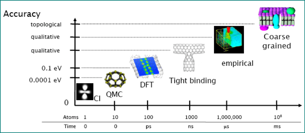
# - My examples are from atomistic materials modelling and electronic structure, but approach is general
# - All the activities I'm interested in require *robust*, *automated* coupling of two or more codes
# - For example, my current projects include:
# - developing and applying multiscale methods
# - generating interatomic potentials
# - uncertainty quantification
#
#
# ## Motivation
#
# - My examples are from atomistic materials modelling and electronic structure, but approach is general
# - All the activities I'm interested in require *robust*, *automated* coupling of two or more codes
# - For example, my current projects include:
# - developing and applying multiscale methods
# - generating interatomic potentials
# - uncertainty quantification
#
#  # ## Case study - concurrent coupling of density functional theory and interatomic potentials
#
#
# ## Case study - concurrent coupling of density functional theory and interatomic potentials
#
# 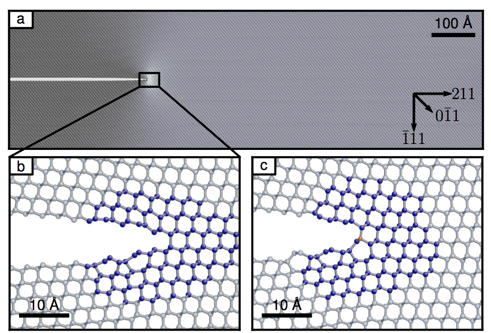 #
# *J.R. Kermode, L. Ben-Bashat, F. Atrash, J.J. Cilliers, D. Sherman and A. De Vita, [Macroscopic scattering of cracks initiated at single impurity atoms.](http://www.nature.com/ncomms/2013/130912/ncomms3441/full/ncomms3441.html) Nat. Commun. 4, 2441 (2013).*
#
# - File-based communication good enough for many projects that combine codes
# - Here, efficient simlulations require a programmatic interface between QM and MM codes
# - Keeping previous solution in memory, wavefunction extrapolation, etc.
# - In general, deep interfaces approach bring much wider benefits
# # Benefits of Scripting Interfaces
#
# **Primary:**
# - Automated preparation of input files
# - Analysis and post-processing
# - Batch processing
#
# **Secondary:**
# - Expand access to advanced feautures to less experienced programmers
# - Simplify too-level programs
# - Unit and regression testing framework
#
# **Longer term benefits:**
# - Encourages good software engineering in main code - modularity, well defined APIs
# - Speed up development of new algorithms by using an appropriate mixture of high- and low-level languages
#
# # Python scripting for interoperability
#
# - Python has emerged as *de facto* "glue" language for atomistic simulations
# - [numpy](http://www.numpy.org/)/[scipy](http://scipy.org/) ecosystem
# - [Matplotlib](http://matplotlib.org/) plotting/interactive graphics
# - [Jupyter](https://jupyter.org/)/IPython notebooks encourage reproducible research
# - [Anaconda](https://jupyter.org/) distribution and package management system
#
# 
#
# http://www.scipy.org
# ## Atomic Simulation Environment (ASE)
#
# - Within atomistic modelling, standard for scripting interfaces is ASE
# - Wide range of calculators, flexible (but not too flexible) data model
# - Can use many codes as drop-in replacements
# - Collection of parsers aids validation and verification (cf. DFT $\Delta$-code project)
# - Coupling $N$ codes requires maintaining $N$ parsers/interfaces to be maintained, not $N^2$ input-output converters
# - High-level functionality can be coded generically, or imported from other packages (e.g. `spglib`, `phonopy`) using minimal ASE-compatible API
#
# https://wiki.fysik.dtu.dk/ase/
# ## QUIP - **QU**antum mechanics and **I**nteratomic **P**otentials
#
# - General-purpose library to manipulate atomic configurations, grew up in parallel with ASE
# - Includes interatomic potentials, tight binding, external codes such as Castep
# - Developed at Cambridge, NRL and King's College London over $\sim10$ years
# - Started off as a pure Fortran 95 code, but recently been doing more and more in Python
# - `QUIP` has a full, deep Python interface, `quippy`, auto-generated from Fortran code using `f90wrap`, giving access to all public subroutines, derived types (classes) and data
#
# 
#
# http://libatoms.github.io/QUIP
# ## Interactive demonstations
#
# - Using live IPython notebook linked to local Python kernel - could also be remote parallel cluster
# - Static view of notebook can be rendered as `.html` or `.pdf`, or as executable Python script
# In[57]:
get_ipython().run_line_magic('pylab', 'inline')
import numpy as np
from chemview import enable_notebook
from matscipy.visualise import view
enable_notebook()
# ## Example: vacancy formation energy in silicon
#
# - Typical example workflow, albeit simplified
# - Couples several tools
# - Generate structure with ASE lattice tools
# - Stillinger-Weber potential implementation from QUIP
# - Relaxations with generic LBFGS optimiser from ASE
# In[58]:
from ase.lattice import bulk
from ase.optimize import LBFGSLineSearch
from quippy.potential import Potential
si = bulk('Si', a=5.44, cubic=True)
sw_pot = Potential('IP SW') # call into Fortran code
si.set_calculator(sw_pot)
e_bulk_per_atom = si.get_potential_energy()/len(si)
vac = si * (3, 3, 3)
del vac[len(vac)/2]
vac.set_calculator(sw_pot)
p0 = vac.get_positions()
opt = LBFGSLineSearch(vac)
opt.run(fmax=1e-3)
p1 = vac.get_positions()
u = p1 - p0
e_vac = vac.get_potential_energy()
print 'SW vacancy formation energy', e_vac - e_bulk_per_atom*len(vac), 'eV'
# # Inline visualisation
# - Chemview IPython plugin uses WebGL for fast rendering of molecules
# - Didn't have an ASE interface, but was quick and easy to add one (~15 lines of code)
# In[59]:
view(vac, np.sqrt(u**2).sum(axis=1), bonds=False)
# ## DFT example - persistent connection, checkpointing
#
# - Doing MD or minimisation within a DFT code typically much faster than repeated single-point calls
# - `SocketCalculator` from `matscipy` package keeps code running, feeding it new configurations via POSIX sockets (local or remote)
# - Use high-level algorithms to move the atoms in complex ways, but still take advantage of internal optimisations like wavefunction extrapolation
# - Checkpointing after each force or energy call allows seamless continuation of complex workflows
# - Same Python script can be submitted as jobscript on cluster and run on laptop
# In[60]:
import distutils.spawn as spawn
from matscipy.socketcalc import SocketCalculator, VaspClient
from matscipy.checkpoint import CheckpointCalculator
from ase.lattice import bulk
from ase.optimize import FIRE
mpirun = spawn.find_executable('mpirun')
vasp = spawn.find_executable('vasp')
vasp_client = VaspClient(client_id=0, npj=2, ppn=12,
exe=vasp, mpirun=mpirun, parmode='mpi',
lwave=False, lcharg=False, ibrion=13,
xc='PBE', kpts=[2,2,2])
vasp = SocketCalculator(vasp_client)
chk_vasp = CheckpointCalculator(vasp, 'vasp_checkpoint.db')
si = bulk('Si', a=5.44, cubic=True)
si.set_calculator(chk_vasp)
e_bulk_per_atom = si.get_potential_energy()/len(si)
vac3 = si.copy()
del vac3[0]
vac3.set_calculator(chk_vasp)
opt = FIRE(vac3)
opt.run(fmax=1e-3)
e_vac3 = vac3.get_potential_energy()
print 'VASP vacancy formation energy', e_vac3 - e_bulk_per_atom*len(vac3), 'eV'
# ## File-based interfaces vs. Native interfaces
#
# - ASE provides file-based interfaces to a number of codes - useful for high throughput
# - However, file-based interfaces to electronic structure codes can be slow and/or incomplete and parsers are hard to keep up to date and robust
# - Standardised output (e.g. chemical markup language, XML) and robust parsers are part of solution
# - [NoMaD Centre of Excellence](http://nomad-coe.eu/) will produce parsers for top ~40 atomistic codes
# - Alternative: native interfaces provide a much deeper wrapping, exposing full public API of code to script writers
# - e.g. GPAW, LAMMPSlib, new Castep Python interface
#
# 
# ## Fortran/Python interfacing
#
# - Despite recent increases in use of high-level languages, there's still lots of high-quality Fortran code around
# - Adding "deep" Python interfaces to existing codes is another approach
# - Future proofing: anything accessible from Python is available from other high-level languages too (e.g. Julia)
#
#
#
# *J.R. Kermode, L. Ben-Bashat, F. Atrash, J.J. Cilliers, D. Sherman and A. De Vita, [Macroscopic scattering of cracks initiated at single impurity atoms.](http://www.nature.com/ncomms/2013/130912/ncomms3441/full/ncomms3441.html) Nat. Commun. 4, 2441 (2013).*
#
# - File-based communication good enough for many projects that combine codes
# - Here, efficient simlulations require a programmatic interface between QM and MM codes
# - Keeping previous solution in memory, wavefunction extrapolation, etc.
# - In general, deep interfaces approach bring much wider benefits
# # Benefits of Scripting Interfaces
#
# **Primary:**
# - Automated preparation of input files
# - Analysis and post-processing
# - Batch processing
#
# **Secondary:**
# - Expand access to advanced feautures to less experienced programmers
# - Simplify too-level programs
# - Unit and regression testing framework
#
# **Longer term benefits:**
# - Encourages good software engineering in main code - modularity, well defined APIs
# - Speed up development of new algorithms by using an appropriate mixture of high- and low-level languages
#
# # Python scripting for interoperability
#
# - Python has emerged as *de facto* "glue" language for atomistic simulations
# - [numpy](http://www.numpy.org/)/[scipy](http://scipy.org/) ecosystem
# - [Matplotlib](http://matplotlib.org/) plotting/interactive graphics
# - [Jupyter](https://jupyter.org/)/IPython notebooks encourage reproducible research
# - [Anaconda](https://jupyter.org/) distribution and package management system
#
# 
#
# http://www.scipy.org
# ## Atomic Simulation Environment (ASE)
#
# - Within atomistic modelling, standard for scripting interfaces is ASE
# - Wide range of calculators, flexible (but not too flexible) data model
# - Can use many codes as drop-in replacements
# - Collection of parsers aids validation and verification (cf. DFT $\Delta$-code project)
# - Coupling $N$ codes requires maintaining $N$ parsers/interfaces to be maintained, not $N^2$ input-output converters
# - High-level functionality can be coded generically, or imported from other packages (e.g. `spglib`, `phonopy`) using minimal ASE-compatible API
#
# https://wiki.fysik.dtu.dk/ase/
# ## QUIP - **QU**antum mechanics and **I**nteratomic **P**otentials
#
# - General-purpose library to manipulate atomic configurations, grew up in parallel with ASE
# - Includes interatomic potentials, tight binding, external codes such as Castep
# - Developed at Cambridge, NRL and King's College London over $\sim10$ years
# - Started off as a pure Fortran 95 code, but recently been doing more and more in Python
# - `QUIP` has a full, deep Python interface, `quippy`, auto-generated from Fortran code using `f90wrap`, giving access to all public subroutines, derived types (classes) and data
#
# 
#
# http://libatoms.github.io/QUIP
# ## Interactive demonstations
#
# - Using live IPython notebook linked to local Python kernel - could also be remote parallel cluster
# - Static view of notebook can be rendered as `.html` or `.pdf`, or as executable Python script
# In[57]:
get_ipython().run_line_magic('pylab', 'inline')
import numpy as np
from chemview import enable_notebook
from matscipy.visualise import view
enable_notebook()
# ## Example: vacancy formation energy in silicon
#
# - Typical example workflow, albeit simplified
# - Couples several tools
# - Generate structure with ASE lattice tools
# - Stillinger-Weber potential implementation from QUIP
# - Relaxations with generic LBFGS optimiser from ASE
# In[58]:
from ase.lattice import bulk
from ase.optimize import LBFGSLineSearch
from quippy.potential import Potential
si = bulk('Si', a=5.44, cubic=True)
sw_pot = Potential('IP SW') # call into Fortran code
si.set_calculator(sw_pot)
e_bulk_per_atom = si.get_potential_energy()/len(si)
vac = si * (3, 3, 3)
del vac[len(vac)/2]
vac.set_calculator(sw_pot)
p0 = vac.get_positions()
opt = LBFGSLineSearch(vac)
opt.run(fmax=1e-3)
p1 = vac.get_positions()
u = p1 - p0
e_vac = vac.get_potential_energy()
print 'SW vacancy formation energy', e_vac - e_bulk_per_atom*len(vac), 'eV'
# # Inline visualisation
# - Chemview IPython plugin uses WebGL for fast rendering of molecules
# - Didn't have an ASE interface, but was quick and easy to add one (~15 lines of code)
# In[59]:
view(vac, np.sqrt(u**2).sum(axis=1), bonds=False)
# ## DFT example - persistent connection, checkpointing
#
# - Doing MD or minimisation within a DFT code typically much faster than repeated single-point calls
# - `SocketCalculator` from `matscipy` package keeps code running, feeding it new configurations via POSIX sockets (local or remote)
# - Use high-level algorithms to move the atoms in complex ways, but still take advantage of internal optimisations like wavefunction extrapolation
# - Checkpointing after each force or energy call allows seamless continuation of complex workflows
# - Same Python script can be submitted as jobscript on cluster and run on laptop
# In[60]:
import distutils.spawn as spawn
from matscipy.socketcalc import SocketCalculator, VaspClient
from matscipy.checkpoint import CheckpointCalculator
from ase.lattice import bulk
from ase.optimize import FIRE
mpirun = spawn.find_executable('mpirun')
vasp = spawn.find_executable('vasp')
vasp_client = VaspClient(client_id=0, npj=2, ppn=12,
exe=vasp, mpirun=mpirun, parmode='mpi',
lwave=False, lcharg=False, ibrion=13,
xc='PBE', kpts=[2,2,2])
vasp = SocketCalculator(vasp_client)
chk_vasp = CheckpointCalculator(vasp, 'vasp_checkpoint.db')
si = bulk('Si', a=5.44, cubic=True)
si.set_calculator(chk_vasp)
e_bulk_per_atom = si.get_potential_energy()/len(si)
vac3 = si.copy()
del vac3[0]
vac3.set_calculator(chk_vasp)
opt = FIRE(vac3)
opt.run(fmax=1e-3)
e_vac3 = vac3.get_potential_energy()
print 'VASP vacancy formation energy', e_vac3 - e_bulk_per_atom*len(vac3), 'eV'
# ## File-based interfaces vs. Native interfaces
#
# - ASE provides file-based interfaces to a number of codes - useful for high throughput
# - However, file-based interfaces to electronic structure codes can be slow and/or incomplete and parsers are hard to keep up to date and robust
# - Standardised output (e.g. chemical markup language, XML) and robust parsers are part of solution
# - [NoMaD Centre of Excellence](http://nomad-coe.eu/) will produce parsers for top ~40 atomistic codes
# - Alternative: native interfaces provide a much deeper wrapping, exposing full public API of code to script writers
# - e.g. GPAW, LAMMPSlib, new Castep Python interface
#
# 
# ## Fortran/Python interfacing
#
# - Despite recent increases in use of high-level languages, there's still lots of high-quality Fortran code around
# - Adding "deep" Python interfaces to existing codes is another approach
# - Future proofing: anything accessible from Python is available from other high-level languages too (e.g. Julia)
#
#  #
#
# # `f90wrap` adds derived type support to `f2py`
#
# - There are many automatic interface generators for C++ codes (e.g. SWIG or Boost.Python), but not many support modern Fortran
# - [f2py](https://sysbio.ioc.ee/projects/f2py2e/) scans Fortran 77/90/95 codes, generates Python interfaces
# - Great for individual routines or simple codes: portable, compiler independent, good array support
# - No support for modern Fortran features: derived types, overloaded interfaces
# - Number of follow up projects, none had all features we needed
# - `f90wrap` addresses this by generating an additional layer of wrappers
# - Supports derived types, module data, efficient array access, Python 2.6+ and 3.x
#
# https://github.com/jameskermode/f90wrap
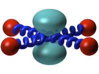
# # Example: wrapping the `bader` code
#
# - Widely used code for post-processing charge densities to construct Bader volumes
# - Python interface would allow code to be used as part of workflows without needing file format converters, I/O, etc.
# - Downloaded [source](http://theory.cm.utexas.edu/henkelman/code/bader/), used `f90wrap` to *automatically* generate a deep Python interface with very little manual work
#
# Generation and compilation of wrappers:
#
# f90wrap -v -k kind_map -I init.py -m bader \
# kind_mod.f90 matrix_mod.f90 \
# ions_mod.f90 options_mod.f90 charge_mod.f90 \
# chgcar_mod.f90 cube_mod.f90 io_mod.f90 \
# bader_mod.f90 voronoi_mod.f90 multipole_mod.f90
#
# f2py-f90wrap -c -m _bader f90wrap_*.f90 -L. -lbader
# In[61]:
from gpaw import restart
si, gpaw = restart('si-vac.gpw')
rho = gpaw.get_pseudo_density()
# In[62]:
atom = 5
plot(si.positions[:, 0], si.positions[:, 1], 'k.', ms=20)
plot(si.positions[atom, 0], si.positions[5, 1], 'g.', ms=20)
imshow(rho[:,:,0], extent=[0, si.cell[0,0], 0, si.cell[1,1]])
# In[63]:
import bader
bdr = bader.bader(si, rho)
# In[66]:
bdr.nvols
# In[67]:
# collect Bader volumes associated with atom #5
mask = np.zeros_like(rho, dtype=bool)
for v in (bdr.nnion == atom+1).nonzero()[0]:
mask[bdr.volnum == v+1] = True
plot(si.positions[:, 0], si.positions[:, 1], 'k.', ms=20)
plot(si.positions[atom, 0], si.positions[5, 1], 'g.', ms=20)
imshow(rho[:,:,0], extent=[0, si.cell[0,0], 0, si.cell[1,1]])
imshow(mask[:,:,0], extent=[0, si.cell[0,0], 0, si.cell[1,1]], alpha=.6)
# # Wrapping Castep with f90wrap
#
# - `f90wrap` can now wrap large and complex codes like the Castep electronic structure code, providing deep access to internal data on-the-fly
# - Summer internship by Greg Corbett at STFC in 2014 produced proof-of-principle implementation
# - Results described in [RAL technical report](https://epubs.stfc.ac.uk/work/18048381)
# - Since then I've tidied it up a little and added a minimal high-level ASE-compatibility layer, but there's plenty more still to be done
#
# 
# ## Current Features
#
# - Implemented in Castep development release:
# make python
# - Restricted set of source files currently wrapped, can be easily expanded.
# Utility: constants.F90 algor.F90
# comms.serial.F90
# io.F90 trace.F90
# license.F90 buildinfo.f90
# Fundamental: parameters.F90 cell.F90 basis.F90
# ion.F90 density.F90 wave.F90
# Functional: model.F90 electronic.F90 firstd.f90
#
# - Already **far** too much to wrap by hand!
# - 35 kLOC Fortran and 55 kLOC Python auto-generated
# - 23 derived types
# - ~2600 subroutines/functions
# ## What is wrapped?
# - Module-level variables: `current_cell`, etc.
# - Fortran derived types visible as Python classes: e.g. `Unit_Cell`
# - Arrays (including arrays of derived types) - no copying necessary to access/modify data in numerical arrays e.g. `current_cell%ionic_positions`
# - Documentation strings extracted from source code
# - Dynamic introspection of data and objects
# - Error catching: `io_abort()` raises `RuntimeError` exception, allowing post mortem debugging
# - Minimal ASE-compatible high level interface
# # Test drive
# In[68]:
import castep
# In[69]:
#castep.
#castep.cell.Unit_Cell.
get_ipython().run_line_magic('pinfo', 'castep.model.model_wave_read')
# ## Single point calculation
# In[70]:
from ase.lattice.cubic import Diamond
atoms = Diamond('Si')
calc = castep.calculator.CastepCalculator(atoms=atoms)
atoms.set_calculator(calc)
e = atoms.get_potential_energy()
f = atoms.get_forces()
print 'Energy', e, 'eV'
print 'Forces (eV/A):'
print f
# ## Interactive introspection
# In[74]:
#calc.model.eigenvalues
#calc.model.wvfn.coeffs
#calc.model.cell.ionic_positions.T
#calc.model.wvfn.
#calc.parameters.cut_off_energy
# In[75]:
figsize(8,6)
plot(castep.ion.get_array_core_radial_charge())
plot(castep.ion.get_array_atomic_radial_charge())
ylim(-0.5,0.5)
# ## Visualise charge density isosurfaces on-the-fly
# In[76]:
# grid points, in Angstrom
real_grid = (castep.basis.get_array_r_real_grid()*
castep.io.io_atomic_to_unit(1.0, 'ang'))
resolution = [castep.basis.get_ngx(),
castep.basis.get_ngy(),
castep.basis.get_ngz()]
origin = np.array([real_grid[i, :].min() for i in range(3)])
extent = np.array([real_grid[i, :].max() for i in range(3)]) - origin
# charge density resulting from SCF
den = calc.model.den.real_charge.copy()
den3 = (den.reshape(resolution, order='F') /
castep.basis.get_total_fine_grid_points())
# visualise system with isosurface of charge density at 0.002
viewer = view(atoms)
viewer.add_isosurface_grid_data(den3, origin, extent, resolution,
isolevel=0.002, color=0x0000ff,
style='solid')
viewer
# ## Postprocessing/steering of running calculations
#
# - Connect Castep and Bader codes without writing any explicit interface or converter
# In[77]:
from display import ListTable
from bader import bader
bdr = bader(atoms, den3)
rows = ListTable()
rows.append(['{0}'.format(hd) for hd in ['Ion', 'Charge', 'Volume']])
for i, (chg, vol) in enumerate(zip(bdr.ionchg, bdr.ionvol)):
rows.append(['{0:.2f}'.format(d) for d in [i, chg, vol] ])
rows
# So far this is just analysis/post-processing, but could easily go beyond this and steer calculations based on results of e.g. Bader analysis.
# ## Updating data inside a running Castep instance
#
# We can move the ions and continue the calculation without having to restart electronic minimisation from scratch (or do any I/O of `.check` files etc.). Here's how the core of the electronic minimisation is coded in Python, almost entirely calling auto-generated routines:
#
# ```python
# new_cell = atoms_to_cell(atoms, kpts=self.kpts)
# castep.cell.copy(new_cell, self.current_cell)
# self.model.wvfn.have_beta_phi = False
# castep.wave.wave_sorthonormalise(self.model.wvfn)
# self.model.total_energy, self.model.converged = \
# electronic_minimisation(self.model.wvfn,
# self.model.den,
# self.model.occ,
# self.model.eigenvalues,
# self.model.fermi_energy)
# self.results['energy'] = io_atomic_to_unit(self.model.total_energy, 'eV')
# ```
# In[78]:
get_ipython().run_line_magic('pinfo', 'castep.wave.wave_orthogonalise')
# ## Example - geometry optimisation
#
# Use embedded Castep efficiently as a standard ASE calculator, giving access to all of the existing high-level algorithms: geometry optimisation, NEB, basin hopping, etc.
# - Compared to file-based interface, save overhead of restarting Castep for each call
# - Reuse electronic model from one ionic configuration to the next
# - Wavefunction and charge density extrapolation possible just as in MD
# In[80]:
from ase.optimize import LBFGS
atoms.rattle(0.01)
opt = LBFGS(atoms)
opt.run(fmax=0.1)
# ## Developing and testing new high-level algorithms
#
# Having a Python interface makes it quick to try out new high-level algorithms.
#
# - e.g. I'm working on a general-purpose preconditioner for geometry optimisation with Christoph Ortner (Warwick), let's try that with Castep
# - This was implemented in a general purpose Python code by Warwick summer student John Woolley, just plug in Castep and off we go!
# In[81]:
from ase.lattice import bulk
import castep
import preconpy.lbfgs as lbfgs
import preconpy.precon as precon
from preconpy.utils import LoggingCalculator
atoms = bulk('Si', cubic=True)
s = atoms.get_scaled_positions()
s[:, 0] *= 0.98
atoms.set_scaled_positions(s)
initial_atoms = atoms
log_calc = LoggingCalculator(None)
for precon, label in zip([None, precon.Exp(A=3, use_pyamg=False)],
['No preconditioner', 'Exp preconditioner']):
print label
atoms = initial_atoms.copy()
calc = castep.calculator.CastepCalculator(atoms=atoms)
log_calc.calculator = calc
log_calc.label = label
atoms.set_calculator(log_calc)
opt = lbfgs.LBFGS(atoms,
precon=precon,
use_line_search=False)
opt.run(fmax=1e-2)
# # Conclusions and Outlook
#
# - Scripting interfaces can be very useful for automating calculations, or connecting components in new ways
# - Can give lecacy C/Fortran code a new lease of life
# - Provides interactive environment for testing, debugging, development and visualisation
# - Appropriate mix of high- and low-level languages maximses overall efficiency
# - **CSC MSc [project](https://www2.warwick.ac.uk/fac/sci/csc/teaching/taughtdegrees/msc/projects/csc-msc-project-jameskermode-pythoncastep.pdf) available on extending Castep/Python interface**
# # Links and References
# - `QUIP` developed with Gábor Csányi, Noam Bernstein, et al.
# - Code https://github.com/libAtoms/QUIP
# - Documentation http://libatoms.github.io/QUIP
# - `matscipy` https://github.com/libAtoms/matscipy, developed with Lars Pastewka, KIT
# - `f90wrap` https://github.com/jameskermode/f90wrap
# - `chemview` https://github.com/gabrielelanaro/chemview/ by Gabriele Lanaro
# - [RAL technical report](https://epubs.stfc.ac.uk/work/18048381) on Castep/Python interface:
# G Corbett, J Kermode, D Jochym and K Refson
#
#
#
# # `f90wrap` adds derived type support to `f2py`
#
# - There are many automatic interface generators for C++ codes (e.g. SWIG or Boost.Python), but not many support modern Fortran
# - [f2py](https://sysbio.ioc.ee/projects/f2py2e/) scans Fortran 77/90/95 codes, generates Python interfaces
# - Great for individual routines or simple codes: portable, compiler independent, good array support
# - No support for modern Fortran features: derived types, overloaded interfaces
# - Number of follow up projects, none had all features we needed
# - `f90wrap` addresses this by generating an additional layer of wrappers
# - Supports derived types, module data, efficient array access, Python 2.6+ and 3.x
#
# https://github.com/jameskermode/f90wrap
# # Example: wrapping the `bader` code
#
# - Widely used code for post-processing charge densities to construct Bader volumes
# - Python interface would allow code to be used as part of workflows without needing file format converters, I/O, etc.
# - Downloaded [source](http://theory.cm.utexas.edu/henkelman/code/bader/), used `f90wrap` to *automatically* generate a deep Python interface with very little manual work
#
# Generation and compilation of wrappers:
#
# f90wrap -v -k kind_map -I init.py -m bader \
# kind_mod.f90 matrix_mod.f90 \
# ions_mod.f90 options_mod.f90 charge_mod.f90 \
# chgcar_mod.f90 cube_mod.f90 io_mod.f90 \
# bader_mod.f90 voronoi_mod.f90 multipole_mod.f90
#
# f2py-f90wrap -c -m _bader f90wrap_*.f90 -L. -lbader
# In[61]:
from gpaw import restart
si, gpaw = restart('si-vac.gpw')
rho = gpaw.get_pseudo_density()
# In[62]:
atom = 5
plot(si.positions[:, 0], si.positions[:, 1], 'k.', ms=20)
plot(si.positions[atom, 0], si.positions[5, 1], 'g.', ms=20)
imshow(rho[:,:,0], extent=[0, si.cell[0,0], 0, si.cell[1,1]])
# In[63]:
import bader
bdr = bader.bader(si, rho)
# In[66]:
bdr.nvols
# In[67]:
# collect Bader volumes associated with atom #5
mask = np.zeros_like(rho, dtype=bool)
for v in (bdr.nnion == atom+1).nonzero()[0]:
mask[bdr.volnum == v+1] = True
plot(si.positions[:, 0], si.positions[:, 1], 'k.', ms=20)
plot(si.positions[atom, 0], si.positions[5, 1], 'g.', ms=20)
imshow(rho[:,:,0], extent=[0, si.cell[0,0], 0, si.cell[1,1]])
imshow(mask[:,:,0], extent=[0, si.cell[0,0], 0, si.cell[1,1]], alpha=.6)
# # Wrapping Castep with f90wrap
#
# - `f90wrap` can now wrap large and complex codes like the Castep electronic structure code, providing deep access to internal data on-the-fly
# - Summer internship by Greg Corbett at STFC in 2014 produced proof-of-principle implementation
# - Results described in [RAL technical report](https://epubs.stfc.ac.uk/work/18048381)
# - Since then I've tidied it up a little and added a minimal high-level ASE-compatibility layer, but there's plenty more still to be done
#
# 
# ## Current Features
#
# - Implemented in Castep development release:
# make python
# - Restricted set of source files currently wrapped, can be easily expanded.
# Utility: constants.F90 algor.F90
# comms.serial.F90
# io.F90 trace.F90
# license.F90 buildinfo.f90
# Fundamental: parameters.F90 cell.F90 basis.F90
# ion.F90 density.F90 wave.F90
# Functional: model.F90 electronic.F90 firstd.f90
#
# - Already **far** too much to wrap by hand!
# - 35 kLOC Fortran and 55 kLOC Python auto-generated
# - 23 derived types
# - ~2600 subroutines/functions
# ## What is wrapped?
# - Module-level variables: `current_cell`, etc.
# - Fortran derived types visible as Python classes: e.g. `Unit_Cell`
# - Arrays (including arrays of derived types) - no copying necessary to access/modify data in numerical arrays e.g. `current_cell%ionic_positions`
# - Documentation strings extracted from source code
# - Dynamic introspection of data and objects
# - Error catching: `io_abort()` raises `RuntimeError` exception, allowing post mortem debugging
# - Minimal ASE-compatible high level interface
# # Test drive
# In[68]:
import castep
# In[69]:
#castep.
#castep.cell.Unit_Cell.
get_ipython().run_line_magic('pinfo', 'castep.model.model_wave_read')
# ## Single point calculation
# In[70]:
from ase.lattice.cubic import Diamond
atoms = Diamond('Si')
calc = castep.calculator.CastepCalculator(atoms=atoms)
atoms.set_calculator(calc)
e = atoms.get_potential_energy()
f = atoms.get_forces()
print 'Energy', e, 'eV'
print 'Forces (eV/A):'
print f
# ## Interactive introspection
# In[74]:
#calc.model.eigenvalues
#calc.model.wvfn.coeffs
#calc.model.cell.ionic_positions.T
#calc.model.wvfn.
#calc.parameters.cut_off_energy
# In[75]:
figsize(8,6)
plot(castep.ion.get_array_core_radial_charge())
plot(castep.ion.get_array_atomic_radial_charge())
ylim(-0.5,0.5)
# ## Visualise charge density isosurfaces on-the-fly
# In[76]:
# grid points, in Angstrom
real_grid = (castep.basis.get_array_r_real_grid()*
castep.io.io_atomic_to_unit(1.0, 'ang'))
resolution = [castep.basis.get_ngx(),
castep.basis.get_ngy(),
castep.basis.get_ngz()]
origin = np.array([real_grid[i, :].min() for i in range(3)])
extent = np.array([real_grid[i, :].max() for i in range(3)]) - origin
# charge density resulting from SCF
den = calc.model.den.real_charge.copy()
den3 = (den.reshape(resolution, order='F') /
castep.basis.get_total_fine_grid_points())
# visualise system with isosurface of charge density at 0.002
viewer = view(atoms)
viewer.add_isosurface_grid_data(den3, origin, extent, resolution,
isolevel=0.002, color=0x0000ff,
style='solid')
viewer
# ## Postprocessing/steering of running calculations
#
# - Connect Castep and Bader codes without writing any explicit interface or converter
# In[77]:
from display import ListTable
from bader import bader
bdr = bader(atoms, den3)
rows = ListTable()
rows.append(['{0}'.format(hd) for hd in ['Ion', 'Charge', 'Volume']])
for i, (chg, vol) in enumerate(zip(bdr.ionchg, bdr.ionvol)):
rows.append(['{0:.2f}'.format(d) for d in [i, chg, vol] ])
rows
# So far this is just analysis/post-processing, but could easily go beyond this and steer calculations based on results of e.g. Bader analysis.
# ## Updating data inside a running Castep instance
#
# We can move the ions and continue the calculation without having to restart electronic minimisation from scratch (or do any I/O of `.check` files etc.). Here's how the core of the electronic minimisation is coded in Python, almost entirely calling auto-generated routines:
#
# ```python
# new_cell = atoms_to_cell(atoms, kpts=self.kpts)
# castep.cell.copy(new_cell, self.current_cell)
# self.model.wvfn.have_beta_phi = False
# castep.wave.wave_sorthonormalise(self.model.wvfn)
# self.model.total_energy, self.model.converged = \
# electronic_minimisation(self.model.wvfn,
# self.model.den,
# self.model.occ,
# self.model.eigenvalues,
# self.model.fermi_energy)
# self.results['energy'] = io_atomic_to_unit(self.model.total_energy, 'eV')
# ```
# In[78]:
get_ipython().run_line_magic('pinfo', 'castep.wave.wave_orthogonalise')
# ## Example - geometry optimisation
#
# Use embedded Castep efficiently as a standard ASE calculator, giving access to all of the existing high-level algorithms: geometry optimisation, NEB, basin hopping, etc.
# - Compared to file-based interface, save overhead of restarting Castep for each call
# - Reuse electronic model from one ionic configuration to the next
# - Wavefunction and charge density extrapolation possible just as in MD
# In[80]:
from ase.optimize import LBFGS
atoms.rattle(0.01)
opt = LBFGS(atoms)
opt.run(fmax=0.1)
# ## Developing and testing new high-level algorithms
#
# Having a Python interface makes it quick to try out new high-level algorithms.
#
# - e.g. I'm working on a general-purpose preconditioner for geometry optimisation with Christoph Ortner (Warwick), let's try that with Castep
# - This was implemented in a general purpose Python code by Warwick summer student John Woolley, just plug in Castep and off we go!
# In[81]:
from ase.lattice import bulk
import castep
import preconpy.lbfgs as lbfgs
import preconpy.precon as precon
from preconpy.utils import LoggingCalculator
atoms = bulk('Si', cubic=True)
s = atoms.get_scaled_positions()
s[:, 0] *= 0.98
atoms.set_scaled_positions(s)
initial_atoms = atoms
log_calc = LoggingCalculator(None)
for precon, label in zip([None, precon.Exp(A=3, use_pyamg=False)],
['No preconditioner', 'Exp preconditioner']):
print label
atoms = initial_atoms.copy()
calc = castep.calculator.CastepCalculator(atoms=atoms)
log_calc.calculator = calc
log_calc.label = label
atoms.set_calculator(log_calc)
opt = lbfgs.LBFGS(atoms,
precon=precon,
use_line_search=False)
opt.run(fmax=1e-2)
# # Conclusions and Outlook
#
# - Scripting interfaces can be very useful for automating calculations, or connecting components in new ways
# - Can give lecacy C/Fortran code a new lease of life
# - Provides interactive environment for testing, debugging, development and visualisation
# - Appropriate mix of high- and low-level languages maximses overall efficiency
# - **CSC MSc [project](https://www2.warwick.ac.uk/fac/sci/csc/teaching/taughtdegrees/msc/projects/csc-msc-project-jameskermode-pythoncastep.pdf) available on extending Castep/Python interface**
# # Links and References
# - `QUIP` developed with Gábor Csányi, Noam Bernstein, et al.
# - Code https://github.com/libAtoms/QUIP
# - Documentation http://libatoms.github.io/QUIP
# - `matscipy` https://github.com/libAtoms/matscipy, developed with Lars Pastewka, KIT
# - `f90wrap` https://github.com/jameskermode/f90wrap
# - `chemview` https://github.com/gabrielelanaro/chemview/ by Gabriele Lanaro
# - [RAL technical report](https://epubs.stfc.ac.uk/work/18048381) on Castep/Python interface:
# G Corbett, J Kermode, D Jochym and K Refson
#