#!/usr/bin/env python
# coding: utf-8

# In[1]:


get_ipython().run_line_magic('matplotlib', 'inline')
import matplotlib.pyplot as plt, seaborn as sn, numpy as np, pandas as pd
sn.set_context('notebook')


# # 1. A hydrological example
# 
# In the next two notebooks, we're going to illustrate everything we've covered so far using a slightly more realisitc example. In this notebook, we will begin by formulating a basic hydrological model to simulate flows in a small Scottish catchment. The model will be too simplistic for most real-world applications, but I hope it will provide a useful illustration of the modelling process. In the second notebook, we'll use the **[emcee](http://dan.iel.fm/emcee/current/)** Python package to calibrate our model and see what we can learn about its parameters *given some real data*.
# 
# ### 1.1. The study catchment
# 
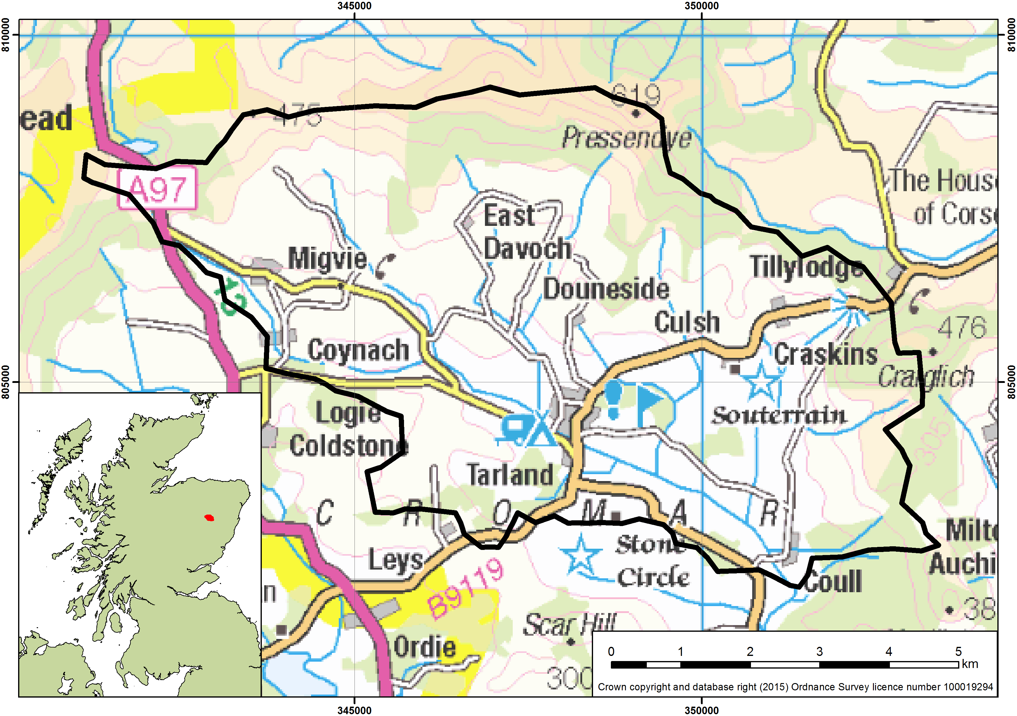
# We're going to use observations from the **Tarland catchment** in Aberdeenshire, Scotland. Flow data are available from 2001 to 2010, together with rainfall and potential evapotranspiration (PET) datasets for the same period that we'll use to drive our model. The catchment has an area of $51.7\,km^2$ and we'll be using flow data from the gauging station at **Coull**.
# 
# <img src="https://github.com/JamesSample/enviro_mod_notes/blob/master/images/Tarland_Map.png?raw=true" alt="Tarland catchment map" width="700"> 
# 
# It is important to stress that *all* these datasets are subject to **error**. For example:
# 
#   1. The **rainfall data** come from spatially interpolated rain gauge measurements. Rain gauges are notoriously inaccurate (especially in Scotland where it's often raining horizontally) and the spatial interpolation process adds further uncertainty <br><br>
#   
#   2. The **PET data** have been estimated using the **[FAO56 modified Penman-Monteith method]('http://www.fao.org/docrep/x0490e/x0490e00.htm')**. This is a whole model in itself, incorporating data on cloud cover, solar radiation, humidity, wind speed, temperature etc., all of which are imperfectly measured. The version of the method used here also assumes the land cover is uniform grass of an even height, which is not the case in the Tarland catchment <br><br>
#   
#   3. The **flow data** are based on an empirically derived **[stage-discharge relationship]('http://water.usgs.gov/edu/streamflow3.html')** which is subject to considerable uncertainty due to changing riverbed sediments and limited gauging data, especially for high flows
#   
# Understanding the limitations of the data is important and in a more comprehensive analysis we might attempt to incorporate uncertainty about our input and calibration data into our likelihood function. Even if we do not do this, we should certainly spend some time **quality checking** the data and perhaps **cleaning or removing points that are obviously spurious**. For the simple example presented here, we will *ignore all these issues* and instead focus only on the **parameter-related uncertainty** in our model. This is an important omission, but I want to keep this example as simple as possible.
# 
# The precipitation and flow data have a **daily** time step, whereas the PET data are **monthly**. For now, we'll simply assume the monthly PET totals are distributed evenly over each day of the month.
# 
# Note that throughout this entire analysis, all water **volumes** will be expressed in **millimetres**. This is not a mistake - we're simply performing all the calculations **per unit area** so we can visualise what's going on in terms of a 1D conceptualisation (see below). In reality, the Tarland catchment has an area of $51.7 \, km^2$, so a rainfall input of 1 mm equates to an actual water volume of $1 \times 10^{-3} * 51.7 \times 10^6 = 51.7 \times 10^3 \, m^3$. 

# In[2]:


# Download Tarland data into a Pandas dataframe
data_url = r'https://raw.githubusercontent.com/JamesSample/enviro_mod_notes/master/data/Tarland_Flow_And_Met_Data.csv'
met_df = pd.read_csv(data_url, parse_dates=True, index_col=0)

# Convert cumecs to mm
cat_area = 51.7E6 # Catchment area in m2
met_df['Runoff_mm'] = met_df['Q_Cumecs']*60*60*24*1000/cat_area
del met_df['Q_Cumecs']

# Linear interpolation of any missing values
met_df.interpolate(method='linear', inplace=True) 

print met_df.head()

# Calculate annual averages for rainfall, PET and runoff
ann_df = met_df.resample('A', how='sum')
print '\nAnnual averages:'
print ann_df.mean()


# Broadly speaking, these annual averages are about what would be expected for a catchment like the Tarland in Eastern Scotland, with the exception that the PET losses look rather too high. This could be because the FAO56 PET calculation (linked above) assumes the land cover is grass with no moisture stress, whereas the actual land cover in the Tarland is mixture of agriculture, forestry, rough grazing and upland vegetation. For comparison, according to the **[UK Hydrometric Register]('http://nora.nerc.ac.uk/3093/1/HydrometricRegister_Final_WithCovers.pdf')**, the Girnock Burn at Littlemill (a little to the southwest of the Tarland) has a long term average annual rainfall of $998 \, mm$ and a mean annual runoff of $554 \, mm$. This means the **actual evapotranspiration (AET)** (plus other losses) accounts for around $454 \, mm$ per year. For Tarland, we're not going to worry about this too much, but we will build a simple *correction factor* into our model to modify the unreasonably high rate of PET.
# 
# ### 1.2. A conceptual hydrological model
# 
# We are going to represent the entire Tarland catchment as **two connected "buckets"**, one representing the **soil water** reservoir and the other representing the **groundwater**. This approach is very common in hydrology, except most practically useful models break the system down into more buckets. For example, some models use different buckets for different combinations of land cover and soil type (often called "**hydrological response units**"); others divide the subsurface into more than two reservoirs, by having e.g. separate "buckets" for shallow versus deep groundwater, and perhaps the same for soil water too. There are many variations on this theme, and once you have lots of buckets there are numerous ways of linking them together, which leads to consideration of e.g. water travel times along different river reaches and between different water stores. 
# 
# All this adds to the complexity of the model and can quickly lead to **over-parameterisation** (as described in notebook 2). We're going to *ignore all of these complexities as well* and just consider two simple buckets. With such a basic setup we certainly can't be accused of over-parameterisation, but equally it's unlikely that this model will be very informative in terms of understanding the hydrology of the Tarland catchment.
# 
# <img src="https://github.com/JamesSample/enviro_mod_notes/blob/master/images/Two_Bucket_Model.png?raw=true" alt="Two bucket model" width="400"> 
# 
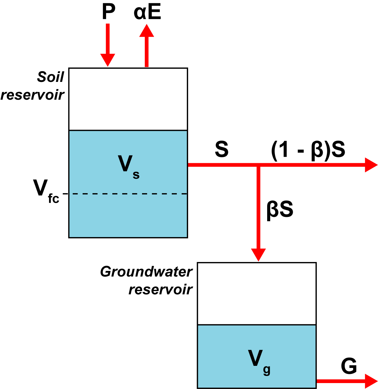# #### Soil reservoir
# 
# For the soil reservoir, we will assume the only water input is the precipitation, $P$. The outputs are **potential** evapotranspiration, $\alpha E$, and soil drainage, $S$. $\alpha$ is a correction factor between $0$ and $1$, which we will use to reduce the Penman-Monteith PET rates to more realistic values. Because we don't know what an appropriate value for $\alpha$ should be, we will include it as a parameter in our calibration procedure.
# 
# The soil reservoir has a **[field capacity](https://en.wikipedia.org/wiki/Field_capacity)**, $V_{fc}$, which is the amount of water the soil "likes to hold onto" under freely draining conditions. We will assume that soil drainage only takes place when the water level in the soil is greater than the field capacity i.e. when $V_s > V_{fc}$. Below field capacity no drainage will take place, but water can still be removed from the soil by evapotranspiration. 
# 
# We will further assume that the soil drainage, $S$, is directly proportional to the volume of water *above field capacity*. The constant of proportionality in this relationship is $\frac{1}{\tau_s}$, where $\tau_s$ is known as the **soil water residence time**. This is the average length of time (in days) that a molecule of water spends in the soil between flowing in and flowing out.
# 
# $$S = \frac{(V_s - V_{fc})}{\tau_s}$$
# 
# [As an aside, it's worth mentioning that this assumption has at least some physical basis: the equation represents the behaviour of a bucket with a hole in the bottom **filled with some porous material** (e.g. soil or sediment) such that the flow of water through the hole is **laminar**. Note that without the porous material the equation would be different.]
# 
# The equation above suggests negative values for $S$ whenever $V_s$ is below field capacity, which is undesirable. To correct for this, we will introduce a function, $g(V_s)$, to set the soil drainage to zero when $V_s < V_{fc}$. One obvious choice for $g(V_s)$ would be
# 
# $$g(V_s) = 0 \qquad for \qquad V_s \leq V_{fc}$$
# $$g(V_s) = 1 \qquad for \qquad V_s > V_{fc}$$
# 
# However, this would introduce non-differentiable discontinuities that could cause problems later. Instead, we can use the **[sigmoid function](https://en.wikipedia.org/wiki/Sigmoid_function)**, which has the form
# 
# $$g(V_s) = \frac{1}{1 + e^{a - V_s}}$$
# 
# If we set the constant $a$ in this equation equal to the field capacity, we obtain a curve which switches very rapidly from approximately zero to approximately 1 when $V_s = V_{fc}$. Based on information in the **[Hydrology of Soil Types (HOST)](http://www.ceh.ac.uk/services/hydrology-soil-types-1km-grid)** database, the average field capacity of soils across the Tarland as a whole is roughly $290 \; mm$.

# In[3]:


# Sigmoid function

fc = 290 # Field capacity (mm)

Vs = np.arange(0, 500, 0.1)
g_Vs = 1/(1 + np.exp(fc - Vs))

plt.plot(Vs, g_Vs, 'r-', label='Sigmoid function')
plt.axvline(fc, c='k', label='Tarland field capacity')
plt.xlabel('$V_s$')
plt.legend(loc='best')
plt.show()


# This version of $g(V_s)$ has the advantaged of being differentiable. We can therefore define the outflow from the soil reservoir, $S$, as
# 
# $$S = \frac{(V_s - V_{fc})}{\tau_s}g(V_s) = \frac{(V_s - V_{fc})}{\tau_s(1 + e^{V_{fc} - V_s})}$$
# 
# Additionally we know that, in reality, **actual** evapotranspiration (AET) differs from **potential** evapotranspiration (PET). One reason for this is that, as the soil dries out, it becomes increasingly difficult to evaporate more water i.e. it is easier to evaporate $1 \; mm$ of water from a wet soil than from a nearly-dry soil. It is often assumed that moisture-limited evapotranspiration begins when the water level falls below field capacity. To represent this in our model we will include an additional correction factor for PET that is a function of soil moisture, $f(V_s)$. In terms of choosing an appropriate function, we want something that tends to $1$ as $V_s$ approaches $V_{fc}$ and tends to $0$ as $V_s$ tends to $0$. Two possible choices are:
# 
# $$f(V_s) = 1 - e^{-\mu V_s} \qquad or \qquad f(V_s) = \frac{V_s}{\mu + V_s}$$
# 
# where $\mu$ is a tuning parameter that determines the shape of the curves. If we calculate AET as $\alpha E f(V_s)$ you should be able to see that, for either of the above choices for $f(V_s)$, when the soil is wet AET will be similar to PET, but as the soil dries out AET is progressively reduced, even if $\alpha E$ remains large.
# 
# For this example we will use the first (exponential) option for $f(V_s)$, and will attempt to choose a value for $\mu$ that is consistent with the soil properties of the Tarland catchment.   The image below superimposes the average field capacity (vertical black line) on a plot of $f(V_s) = 1 - e^{-\mu V_s}$ for a range of values of $\mu$.

# In[4]:


mus = np.arange(0.01, 0.05, 0.005) # Selection of values for mu
Vs = np.arange(0, 500, 0.5)        # Vs from 0 to above field capacity
fc = 290  # Field capacity (mm)

# Loop over mu values
for mu in mus:
    f_Vs = 1 - np.exp(-mu*Vs)
    plt.plot(Vs, f_Vs, label='mu = %.3f' % mu)

plt.axvline(fc, c='k')
plt.legend(loc='best')
plt.ylabel('$f(V_s)$')
plt.xlabel('$V_s$')
plt.show()


# For the lower curve on this plot ($\mu = 0.01$), moisture limitation begins too soon: $f(V_s)$ is significantly below 1 even when the water level is well above field capacity. On the other hand, when $\mu = 0.04$, moisture limitation does not really begin until $V_s \approx 100 \; mm$, which is too low. Based on this rough investigation, $\mu = 0.02$ seems like a reasonable choice in this case because 
# 
# $$f(V_s) \approx 1 \qquad for \qquad V_s > V_{fc}$$
# $$f(V_s) < 1 \qquad for \qquad V_s < V_{fc}$$
# 
# For the volume of water in the soil reservoir, we can therefore write the following differential equation based on balancing inputs and outputs
# 
# $$\frac{dV_s}{dt} = P - \alpha E (1 - e^{-0.02V_s}) - S$$
# 
# Ideally, however, we would like an equation for $\frac{dS}{dt}$, because we would like to know the amount of water leaving the soil to either the groundwater or the stream. Finding $\frac{dS}{dt}$ is not straightforward but, using the **[chain rule](https://en.wikipedia.org/wiki/Chain_rule)**, we know that
# 
# $$\frac{dS}{dt} = \frac{dV_s}{dt} \frac{dS}{dV_s}$$
# 
# We have just written down an equation for $\frac{dV_s}{dt}$ and, from the discussion above, we also have an equation for $S$ in terms of $V_s$, which we can differentiate to give $\frac{dS}{dV_s}$. The differential can be calculated by hand using the **[product rule](https://en.wikipedia.org/wiki/Product_rule)** or, if you're feeling lazy, you can always try **[Wolfram Alpha](http://www.wolframalpha.com/input/?i=derivative+%28x-+a%29%2F%28b*%281+%2B+exp%28a+-+x%29%29%29)** instead. The result is that if
# 
# $$S = \frac{(V_s - V_{fc})}{\tau_s(1 + e^{V_{fc} - V_s})}$$
# 
# (from above) then
# 
# $$\frac{dS}{dV_s} = \frac{(V_s - V_{fc})e^{V_{fc} - V_s}}{T_s(e^{V_{fc} - V_s} + 1)^2} + \frac{1}{T_s(e^{V_{fc} - V_s} + 1)}$$
# 
# Although this equation looks pretty horrible, we now have everything we need to simulate the soil water reservoir.
# 
# #### Groundwater reservoir
# 
# For the groundwater reservoir, we assume that a fraction, $\beta$, of the water draining from the soil reservoir moves downwards into the groundwater. The remainder of the soil drainage, $(1 - \beta S)$, is assumed to travel directly to the stream along fast, shallow flow pathways. 
# 
# $\beta$ is sometimes referred to as the **Base Flow Index (BFI)** and it can be estimated in a variety of ways. For the Tarland catchment, previous work suggests that $\beta \approx 0.6$ and, even though there is considerable uncertainty in this value, to keep things simple we will fix $\beta = 0.6$ in our model and will not include it in our calibration procedure.
# 
# The groundwater reservoir behaves in the same way as the soil water reservoir, except it's simpler because we don't need to worry about issues such as evapotranspiration and field capacity. The rate of change of volume in the groundwater is equal to the balance of inputs and outputs
# 
# $$\frac{dV_g}{dt} = \beta S - G$$ 
# 
# and the outflow from the groundwater is directly proportional to the groundwater storage volume
# 
# $$G = \frac{1}{\tau_g}V_g$$
# 
# where $\tau_g$ is the **groundwater residence time**. As above, we are primarily interested in $\frac{dG}{dt}$, which we can calculate using the chain rule
# 
# $$\frac{dG}{dt} = \frac{dV_g}{dt} \frac{dG}{dV_g}$$
# 
# From these equations we can write
# 
# $$\frac{dG}{dt} = \frac{\beta S - G}{T_g}$$
# 
# #### Summary of model equations
# 
# Ultimately, we want to use the model to predict the total runoff volume to the stream, $R$, at each time step
# 
# $$R = D_s + D_g$$
# 
# where $D_s$ and $D_g$ are the soil and groundwater drainage volumes respectively. To find $D_s$ and $D_g$, we must first integrate the differential equations for $\frac{dS}{dt}$ and $\frac{dG}{dt}$ to discover how $S$ and $G$ vary with time i.e. given a set of model inputs, parameters and initial conditions, we can calculate the flow rates from the soil and groundwater reservoirs at any point in time. Furthermore, if we integrate these equations *again* we can calculate the **volume of water** draining from the two boxes within any interval of interest (this is because the area under the flow rate curve is equal to the flow volume).
# 
# To represent all this, we can write down a system of **coupled, first-order Ordinary Differential Equations (ODEs)**
# 
# $$\frac{dV_s}{dt} = P - \alpha E (1 - e^{-0.02V_s}) - S$$
# 
# <br><br>
# 
# $$\frac{dS}{dV_s} = \frac{(V_s - V_{fc})e^{V_{fc} - V_s}}{\tau_s(e^{V_{fc} - V_s} + 1)^2} + \frac{1}{\tau_s(e^{V_{fc} - V_s} + 1)}$$
# 
# <br><br>
# 
# $$\frac{dS}{dt} = \frac{dV_s}{dt} \frac{dS}{dV_s}$$
# 
# <br><br>
# 
# $$\frac{dG}{dt} = \frac{\beta S - G}{\tau_g}$$
# 
# <br><br>
# 
# $$\frac{dD_s}{dt} = (1 - \beta) S$$
# 
# <br><br>
# 
# $$\frac{dD_g}{dt} = G$$
# 
# ### 1.3. Parameterising the model
# 
# Although this is a fairly simple model, we already have several choices to make regarding what to include in our calibration procedure. In the discussion above, we have decided not to explicitly consider errors in the input time series ($P$ and $E$), or in the observed flow data, $R_{obs}$. The model itself has five parameters: $\alpha$, $\beta$, $\tau_s$, $\tau_g$ and $\mu$. We have already decided to fix $\mu = 0.02$ and $\beta = 0.6$. We will **include the remaining three parameters in our calibration procedure**.
# 
# ## 2. Solving ODEs
# 
# Solving systems of ODEs is a large and complicated topic in itself, with quite a few pitfalls for the unwary. Within Python, a variety of tools are available, ranging from the basic solvers in [`scipy.integrate.ode`](http://docs.scipy.org/doc/scipy/reference/generated/scipy.integrate.ode.html), to the more sophisticated options provided by [`odespy`](https://github.com/hplgit/odespy) and the full **dynamic systems modelling** capabilities of [`PyDSTool`](http://www.ni.gsu.edu/~rclewley/PyDSTool/FrontPage.html). For many real-world applications, it may be worth investigating these options in detail, but for the example here we will make use of [`scipy.integrate.odeint`](http://docs.scipy.org/doc/scipy/reference/generated/scipy.integrate.odeint.html), which is probably the simplest interface for solving ODEs in Python.
# 
# We'll begin with an illustration of how to solve our system for a single time step, where $P$ and $E$ are kept constant. At this stage, we'll also choose fixed values for all the calibrating parameters ($\alpha$, $\tau_s$ and $\tau_g$). Note that the idea here is just to illustrate solving the ODE system, not to actually calibrate the model.

# In[5]:


from scipy.integrate import odeint

# Example model parameters
alpha = 0.75    # PET correction factor (dimensionless)
beta = 0.6      # BFI (dimensionless)
T_s = 10.       # Soil residence time (days)
T_g = 100.      # Groundwater residence time (days)
fc = 290        # Field capacity (mm)
step_len = 300  # Time step length (days)

# Example initial conditions
P = 8.         # Precipitation (mm/day)
E = 4.         # PET (mm/day)
Vs0 = 0.       # Initial soil volume (mm)
Vg0 = 0.       # Initial groundwater volume (mm)

# Calculate S0 and G0 from Vs0 and Vg0
S0 = (Vs0 - fc)/(T_s*(1 + np.exp(fc - Vs0)))
G0 = Vg0/T_g       

# Array of time points at which to evaluate ODEs
ti = np.linspace(0, step_len, 1000)

def f(y, t, params):
    """ Define ODE system.
            y is list [V, S, G, Ds, Dg]
            t is an array of time points of interest
            params is a tuple (P, E, alpha, beta, T_s, T_g, fc)
    """
    # Unpack incremental values for S and G
    Vi = y[0]
    Si = y[1]
    Gi = y[2]
    
    # Unpack params
    P, E, alpha, beta, T_s, T_g, fc = params

    # Model equations (see section 2.2)
    dS_dV = (((Vi - fc)*np.exp(fc - Vi))/(T_s*((np.exp(fc-Vi) + 1)**2))) + (1/(T_s*(np.exp(fc-Vi) + 1)))
    dV_dt = P - alpha*E*(1 - np.exp(-0.02*Vi)) - Si
    dS_dt = dS_dV*dV_dt
    dG_dt = (beta*Si - Gi)/T_g
    dDs_dt = (1 - beta)*Si
    dDg_dt = Gi
    
    # Add results of equations to an array
    res = np.array([dV_dt, dS_dt, dG_dt, dDs_dt, dDg_dt])
    
    return res

# Vector of initial conditions
y0 = [Vs0, S0, G0, 0, 0]

# Model parameters
params=[P, E, alpha, beta, T_s, T_g, fc]

# Solve
y = odeint(f, y0, ti, args=(params,))

# Build df from output
df = pd.DataFrame(data=y,
                  columns=['V', 'S', 'G', 'Ds', 'Dg'],
                  index=ti)
df.plot(subplots=True, figsize=(8, 10))
print df.tail()


# It's worth considering these plots in detail to understand what's going on. The soil and groundwaetr buckets are initially empty, and the rates of precipitation and **potential** evapotranspiration are held constant at $8 \; mm/day$ and $4 \; mm/day$, respectively. For PET we also applied a correction factor, $\alpha = 0.75$, so the modified PET rate is actually $3 \; mm/day$. However, because the soil is initially dry, the **actual** evapotranspiration is reduced to **zero** by our correcting function, $f(V_s)$. Also, because the soil water level is below field capacity, the function $g(V_s)$ keeps the soil drainage at zero, so no water drains either to the groundwater reservoir or to the stream. 
# 
# The soil water reservoir therefore begins to fill at a rate that is initially equal to $P$. As soon as the soil becomes wet, AET can also take place at a rate governed by $f(V_s)$, so the soil reservoir continues to fill, but more slowly.
# 
# After a little over $50 \; days$, the soil reaches field capacity and soil drainage begins. At this point, $f(V_s) \approx 1$ and so $AET = PET = 3 \; mm/day$ i.e. evapotranspiration is no longer moisture limited and the net **hydrologically effective rainfall** (precipitation minus AET) is equal to $5 \; mm/day$. As the water level in the soil increases above field capacity, the outflow rate also increases until $S = 5 \; mm/day$, at which point the inputs and outputs are balanced and the soil store achieves equilibrium. The expected steady-state water level can be determined from the equations above: as long as we are above field capacity, we know that
# 
# $$S = \frac{V_s - V_{fc}}{\tau_s}$$
# 
# We therefore expect the soil water level to stabilise at $V_s = S \tau_s + V_{fc}$, which for this example is $340 \; mm$. This is confirmed by the top plot above.
# 
# Once drainage from the soil begins, the water level in the groundwater also starts to rise. In this example, the groundwater reservoir is slower to respond than the soil store ($\tau_g = 100 \; days$; $\tau_s = 10 \; days$), so the outflow rate, $G$, increases more slowly. At equilibrium, the inflow rate to the groundwater is equal to $\beta S = 0.6 \times 5 = 3 \; mm/day$. It is clear from the plot for $G$ that the groundwater outflow rate is slowly approaching this value, but has not quite reached steady-state in the $300$ time steps simulated.
# 
# ## 3. Looping over a time series
# 
# We now have a model that can simulate the evolution of the soil and groundwater stores for any **constant** values of $P$ and $E$. However, we want to drive our model using a daily meteorological time series for the Tarland catchment, so the values of $P$ and $E$ will change from day to day. To allow for this, we will run our model in a loop where the $P$ and $E$ values for the $ith$ iteration are taken from the $ith$ day of the time series. The water level at the end of time step $t_i$ will form the initial conditions for the water level at the start of time step $t_{i+1}$, and for each step we will calculate the total amount of water draining along each of the two flow pathways ($D_s$ and $D_g$).

# In[6]:


def simple_hydro_model(met_df, ics, mod_params, period, step_len=1):
    """ Runs the hydrological model.
    
            met_df         Dataframe containing columns 'Rainfall_mm' and 'PET_mm', with datetime index
            ics            Vector of initial conditions [Vs0, Vg0]
            mod_params     Vector of params [alpha, beta, T_s, T_g, fc]
            period         Vector of [start, end] dates [yyyy-mm-dd, yyyy-mm-dd]
            step_len       Length of each step in the input dataset (days)
        
        Returns a dataframe with column headings
        
            [Vs, S, G, Ds, Dg, Sim_Runoff, Obs_Runoff]
    """
    # Truncate the met data to the desired period
    input_df = met_df.truncate(before=period[0], after=period[1])

    # Unpack initial conditions
    Vs0, Vg0 = ics
    
    # Unpack model parameters
    alpha, beta, T_s, T_g, fc = mod_params
    
    # Time points to evaluate ODEs at. We're only interested in the start and the end of each step
    ti = [0, step_len]

    # List to store output
    output = []

    # Loop over met data
    for idx in range(len(input_df)):
        # Get P and E for this day
        P = input_df.ix[idx, 'Rainfall_mm']
        E = input_df.ix[idx, 'PET_mm']

        # Calculate S0 and G0 from Vs0 and Vg0
        S0 = (Vs0 - fc)/(T_s*(1 + np.exp(fc - Vs0)))
        G0 = Vg0/T_g 

        # Vector of initial conditions
        y0 = [Vs0, S0, G0, 0, 0]

        # Model parameters
        params=[P, E, alpha, beta, T_s, T_g, fc]

        # Solve
        y = odeint(f, y0, ti, args=(params,))

        # Extract values for end of step
        res = y[1]

        # Numerical errors may result in very tiny values <0
        # set these back to 0
        res[res<0] = 0
        output.append(res)

        # Update initial conditions for next step
        Vs0 = res[0]
        Vg0 = res[2]*T_g

    # Build a dataframe of results
    df = pd.DataFrame(data=np.vstack(output),
                      columns=['Vs', 'S', 'G', 'Ds', 'Dg'],
                      index=input_df.index)

    # Estimate runoff as Ds + Dg
    df['Sim_Runoff_mm'] = df['Ds'] + df['Dg']

    # Add observed runoff to df
    df['Obs_Runoff_mm'] = input_df['Runoff_mm']

    return df


# We can now run the model and compare the results to the observations. First, we'll just look at the model outputs for the first year of data.

# In[7]:


# Model setup
# Model parameters
alpha = 0.75          # PET correction factor (dimensionless)
beta = 0.6            # BFI (dimensionless)
T_s = 10.             # Soil residence time (days)
T_g = 100.            # Groundwater residence time (days)
fc = 290              # Field capacity (mm)
st_dt = '2000-01-01'  # Start date
end_dt = '2000-12-31' # End date

# Initial conditions
Vs0 = 0.       # Initial soil volume (mm)
Vg0 = 0.       # Initial groundwater volume (mm)

# Run model
df = simple_hydro_model(met_df=met_df,
                        ics=[Vs0, Vg0],
                        mod_params=[alpha, beta, T_s, T_g, fc],
                        period=[st_dt, end_dt])

# Plot the simulated results
df[['Vs', 'S', 'G', 'Ds', 'Dg']].plot(subplots=True, 
                                      figsize=(8, 10))


# The first thing to notice about this model run is that the soil does not reach field capacity until early September. This is not surprising, as both the soil and groundwater reservoirs were assumed to be *completely dry* at the start of the simulation, which is not realistic. Looking at the top plot, showing the water level in the soil through time, we can see that the level rises steadily from January until about the end of April, and then remains level and even declines slightly throughout much of the summer. The level then begins to rise again during August and remains quite high throughout most of the winter. This all seems fairly reasonable, but it's obvious that the first nine months or so of the simulation are not telling us anything useful about the Tarland catchment. During this period, our model is **equilibrating** and "forgetting" about its arbitrary starting position, as expressed by the initial conditions. It is usual to discard this portion of the simulation before comparing the model output to the observations. This phase is often called the model's "**burn-in period**", and we discard it for exactly the same reasons that we discard the burn-in phase of an MCMC chain (see notebook 4). 
# 
# It is also worth noting from the plots above that the traces for the soil reservoir are much more "spiky" than the ones for the groundwater store. This is because we set the groundwater **residence time**, $\tau_g$ to be ten times bigger than for the soil reservoir, $\tau_s$. The soil reservoir is therefore much more responsive.
# 
# In the example below, we run the model for 5 years, then discard the first year of simulations (as the burn-in period) and compare the remaining 4 years to the observed runoff data.

# In[8]:


# Model setup
# Model parameters
alpha = 0.75          # PET correction factor (dimensionless)
beta = 0.6            # BFI (dimensionless)
T_s = 10.             # Soil residence time (days)
T_g = 100.            # Groundwater residence time (days)
fc = 290              # Field capacity (mm)
st_dt = '2000-01-01'  # Start date
end_dt = '2004-12-31' # End date

# Initial conditions
Vs0 = 0.       # Initial soil volume (mm)
Vg0 = 0.       # Initial groundwater volume (mm)

# Run model
df = simple_hydro_model(met_df=met_df,
                        ics=[Vs0, Vg0],
                        mod_params=[alpha, beta, T_s, T_g, fc],
                        period=[st_dt, end_dt])

# Discard burn-in
df = df.truncate(before='2001-01-01')

df[['Sim_Runoff_mm', 'Obs_Runoff_mm']].plot(alpha=0.5,
                                            figsize=(15, 6))


# For a very first attempt using made-up parameter values this actually isn't too bad. It's reassuring that the model picks up most of the major flow events, even if it doesn't characterise them very accurately. On the other hand, it's obvious that our model is slow to respond compared to the real Tarland system: the observed data is much spikier and has faster recession times than our simulated series.
# 
# In a real modelling application, at this stage it would be a good idea to set aside some time for **manual calibration** (see notebook 2). By manually changing the values for $\alpha$, $\tau_s$ and $\tau_g$ and re-running the code above, it is possible to get a feel for how each paramter influences the model output. This is a very useful step towards a full uncertainty analysis and it's also an excellent way to discover some of the limitations of your model. However, because this is just an illustrative example, we're going to skip manual calibration and go straight to auto-calibration using MCMC (in the next notebook). 
# 
# ## 4. Summary
# 
#   1. Building a physically-based model of a real-world system involves a lot of **simplification and conceptualisation**. <br><br>
#   
#   2. The equations governing physically-based models can often be expressed as systems of **coupled, first-order ordinary differential equations**. In general, these systems are either very difficult or impossible to solve analytically, so we have to rely on **numerical approximations** instead. <br><br>
#   
#   3. Numerically solving systems of ODEs is huge subject. Although fairly simple in principle, in practice there are lots of complications that may lead to inefficient or inaccurate solutions. Things become especially tricky if the system being modelled includes **transitions, thresholds or discontinuities**, which pose problems for most standard numerical solvers. In some cases it may be possible to design the model so as to avoid such problems (as we did above). Otherwise, a **dynamical systems modelling package** may be required to deal with the additional complexity. <br><br>
#   
#   4. Even very simple models can have a surprisingly large number of poorly-constrained parameters. A decision must be made regarding **which ones to include in the uncertainty analysis and which to fix as constants**. Including all the parameters is more rigorous, but will likely lead to parameter identifiability issues unless you have a vast amount of data to calibrate against.