#!/usr/bin/env python
# coding: utf-8

# # Data to Dome: Visualizing Gamma Ray Bursts in WWT

# For this month’s tutorial we will create a visualization of Gamma Ray Bursts. The tutorial was created for A KICP short course for museum and planetarium staff about the Evolving Universe (http://kicp-courses.uchicago.edu/2014/index.php) held this September. Here we will only visualize the data in WWT. While similar visualizations are possible in other planetarium software packages, the process of creating them is somewhat awkward. The time domain is the next great frontier for astronomy, I encourage software vendors to follow along with the tutorial and think about how they can streamline the process of creating a similar visualization using their software.<br><br>
# Mark Subbarao (msubbarao at adlerplanetarium.org)

# ##### Python Setup

# In[1]:


from astropy.table import Table,Column
from astropy.time import Time
from astropy import units
from astropy.coordinates import SkyCoord
from astroquery.vizier import Vizier


# In[2]:


#Create Vizier object, turn off default row limit
v = Vizier()
v.ROW_LIMIT = -1


# ##### WWT Setup

# In[ ]:


from pywwt.mods import *


# In[ ]:


#Connect to WWT
wwt = WWTClient() #Can pass a IP address here if WWT is running on a remote machine
wwt.new_layer_group("Sky","Dynamic Universe")


# ### Gamma Ray Bursts

# For out data catalog we'll choose The second Fermi/GBM GRB catalog (4yr) (von Kienlin+, 2014)
# Vizier catalog: J/ApJS/211/13/GBM
# Which contains Fermi events from July 2007 to July 2012

# In[3]:


Cats = v.get_catalogs('J/ApJS/211/13/GBM')


# In[5]:


Cats[0]


# In[6]:


grbCat=Cats[0]
grbCat.keep_columns(["GRB","RAJ2000","DEJ2000","Time","ObsTime","Fl.w","Fl.n"])
grbCat.rename_column('RAJ2000', 'RA')
grbCat.rename_column('DEJ2000', 'dec')


# In[7]:


grbCat


# In[ ]:


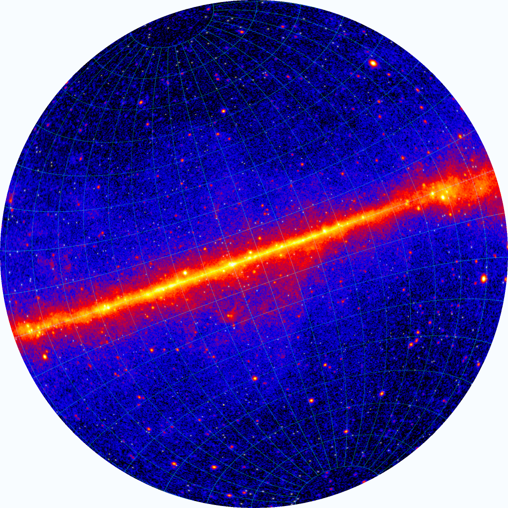
#Plot the Catalog
get_ipython().run_line_magic('config', 'InlineBackend.rc = {}')
import matplotlib
import matplotlib.pyplot as plt
get_ipython().run_line_magic('matplotlib', 'inline')


# In[ ]:


#Plot the Catalog
coordsCol=SkyCoord(grbCat['RA'],grbCat['dec'],'icrs')
fig = plt.figure (figsize=(8,6))
ax = fig.add_subplot(111,projection="mollweide", axisbg='white')
ax.grid(True)
ax.get_xaxis().tick_bottom()
ax.scatter(coordsCol.galactic.l.wrap_at(180.*units.degree).radian,\
           coordsCol.galactic.b.radian,s=6,lw=0)


# Extracting the event time from this table is tricky. The time of day is in the ObsTime column, but the date is embedded in the GRB name. We'll extract the date from the GRB name and combine that with ObsTime to make a astropy time object. 

# In[9]:


timeList=[]
grbList=grbCat['GRB']
for i in range(len(grbList)):
    timeString= grbList[i][2:4].decode()+'/'+grbList[i][4:6].decode()+'/'+'20'+grbList[i][0:2].decode()+' '+grbCat['ObsTime'][i].decode()
    timeList.append(timeString)


# ##### Export Catalog to WWT

# WWT contains its own time format, unfortunately one that astropy cannot write, so we'll have to create our own custom string.

# In[10]:


grbList=grbCat['GRB']
timeList=[]
for i in range(len(grbList)):
    timeString= grbList[i][2:4].decode()+'/'+grbList[i][4:6].decode()+'/'+'20'+grbList[i][0:2].decode()+' '+grbCat['ObsTime'][i].decode()
    timeList.append(timeString)
grbCat.add_column(Column(timeList,name='TimeAndDate'))
grbCat


# In[11]:


#Set up WWT layer
grb_layer = wwt.new_layer("Dynamic Universe", "Gamma Ray Bursts", grbCat.colnames)
#Set visualization parameters in WWT
props_dict = {"CoordinatesType":"Spherical",\
              "MarkerScale":"Screen",\
              "PointScaleType":"Constant",\
              "ScaleFactor":"64",\
              "ShowFarSide":"True",\
              "RaUnits":"Degrees",\
              "PlotType":"Gaussian",\
              "ColorValue":"ARGBColor:255:255:255:255",\
              "TimeSeries":"False"}
grb_layer.set_properties(props_dict)
#Send data to WWT client
grb_layer.update(data=grbCat, purge_all=True, no_purge=False, show=True)


# Now inside WWT we can choose how we visualize the data, we can show all the data at once or playback the events as they happen watching the GRB’s go off like popcorn across the sky. 

# <img src=https://raw.githubusercontent.com/IPSScienceVisualization/python-tutorials/master/images/GRBWWT.png>

# In[ ]: