In [1]:
import pandas as pd
from pandas import Series, DataFrame, Panel
import numpy as np
import datetime
import matplotlib.pyplot as plt
%matplotlib inline
In [2]:
COLUMN_NAMES = ["amount paid", "paid duration mins", "start date", \
                "start day", "end date", "end day", "start time", "end time", \
                "DesignationType", "Hours of Control", "Tariff", "Max Stay", \
                "Spaces", "Street", "x coordinate", "y coordinate", "latitude", \
                "longitude"]
PARKING_DATA = 'ParkingCashlessDenorm.csv'
In [3]:
raw_data = pd.read_csv(PARKING_DATA, names=COLUMN_NAMES, header=None)
raw_data.head()
Out[3]:
| amount paid | paid duration mins | start date | start day | end date | end day | start time | end time | DesignationType | Hours of Control | Tariff | Max Stay | Spaces | Street | x coordinate | y coordinate | latitude | longitude | |
|---|---|---|---|---|---|---|---|---|---|---|---|---|---|---|---|---|---|---|
| 0 | 3.3 | 45 | 2013-02-06 00:00:00 | Wednesday | 2013-02-06 00:00:00 | Wednesday | 10:58 | 11:43 | Shared Use P&D | Mon - Sat 8.30am - 6.30pm | 4.4 | 4 hours | 13 | Hyde Park Square | 527154.134706 | 181061.021077 | 51.514183 | -0.168964 |
| 1 | 4.4 | 60 | 2013-02-06 00:00:00 | Wednesday | 2013-02-06 00:00:00 | Wednesday | 12:44 | 13:44 | Shared Use P&D | Mon - Sat 8.30am - 6.30pm | 4.4 | 4 hours | 13 | Hyde Park Square | 527154.134706 | 181061.021077 | 51.514183 | -0.168964 |
| 2 | 2.4 | 60 | 2013-02-06 00:00:00 | Wednesday | 2013-02-06 00:00:00 | Wednesday | 13:44 | 14:44 | P&D + PbP | Mon - Fri 8.30-6.30 Sat 8.30 - 1.30 | 2.4 | 4 Hours | 13 | Queensborough Terrace | 526036.819680 | 180730.025823 | 51.511458 | -0.185176 |
| 3 | 2.4 | 60 | 2013-06-08 00:00:00 | Saturday | 2013-06-08 00:00:00 | Saturday | 08:43 | 09:43 | P&D + PbP | Mon - Sat 8.30am - 6.30pm | 2.4 | 4 Hours | 15 | Winsland Street | 526709.888753 | 181367.836585 | 51.517040 | -0.175253 |
| 4 | 7.0 | 105 | 2013-06-08 00:00:00 | Saturday | 2013-06-08 00:00:00 | Saturday | 15:44 | 17:29 | P&D + PbP | Mon - Sat 8.30am - 6.30pm | 4 | 4 hours | 5 | Wigmore Street | 528210.089071 | 181233.842719 | 51.515498 | -0.153692 |
In [4]:
# pandas will usually do a good job of interpretting time and date information.
# However, rather annoyingly the date and time data has been stored in separate columns
# so we need to do a bit of work to get consistent timestamps to work with.

# First we convert the date information into timestamp format
# Since no time information is given pandas assumes the time as 00:00:00
raw_data['start date'] = pd.to_datetime(raw_data['start date'])
raw_data['end date'] = pd.to_datetime(raw_data['end date'])

# Next convert the time information into timestamp format
# Since the time information has no date associated with it pandas assumes
# the date is today, so we'll need to subtract today's date to get the time on its own
raw_data['start time'] = pd.to_datetime(raw_data['start time'])
raw_data['end time'] = pd.to_datetime(raw_data['end time'])

# We can now construct a proper timestamp for each of the records by adding
# the date and time and subtracting today's date
ts_today = pd.to_datetime('00:00:00')
raw_data['start time'] = raw_data['start time'] - ts_today
raw_data['end time'] = raw_data['end time'] - ts_today
raw_data['start datetime'] = raw_data['start date'] + raw_data['start time']
raw_data['end datetime'] = raw_data['end date'] + raw_data['end time']
In [ ]:
# i've subsequently realised that the whole of the above code can be replaced with this
rows = pd.read_csv(PARKING_CASHLESS,
					 names=COLUMN_NAMES,
					 header=None,
					 parse_dates={'end datetime': ['end date','end time'] , 'start datetime':['start date','start time']})

# How nice is that!
In [6]:
# Now we want to group together all records for each parking location based on
# the latitude and longitude, the 'Street' is ambiguous since some streets have
# more than one parking location
parking_locations = raw_data.groupby(by = ['latitude', 'longitude'])

# get a single location
df1 = raw_data.ix[parking_locations.indices[parking_locations.indices.keys()[3]]]


arrivals = Series(np.ones(df1.shape[0]), index = df1['start datetime'])
departures = Series(-1*np.ones(df1.shape[0]), index = df1['end datetime'])
arr_dep = arrivals.append(departures)
occupancy = arr_dep.resample('10Min', how ='sum').fillna(0).cumsum()
occupancy.plot(xlim =(occupancy.index[15000],occupancy.index[15200]))
Out[6]:
<matplotlib.axes.AxesSubplot at 0x3da5f470>

In [ ]:
# We now construct a Panel object containing the average occupancy for each day of the week
first_time = 1
for j, k in enumerate(parking_locations.indices.keys()):
    # print j
    # look at one location at a time
    df1 = raw_data.ix[parking_locations.indices[k]]
    # Calculate occupancy by incrementing a count for every arrival and decrementing the
    # same count for every departure
    arrivals = Series(np.ones(df1.shape[0]), index = df1['start datetime'])
    departures = Series(-1*np.ones(df1.shape[0]), index = df1['end datetime'])
    occupancy = arrivals.append(departures)
    occupancy = occupancy.resample('10Min', how = 'sum').fillna(0).cumsum()

    # split the data by day of the week
    mon = occupancy.ix[occupancy.index.dayoftheweek == 0]
    tue = occupancy.ix[occupancy.index.dayoftheweek == 1]
    wed = occupancy.ix[occupancy.index.dayoftheweek == 2]
    thu = occupancy.ix[occupancy.index.dayoftheweek == 3]
    fri = occupancy.ix[occupancy.index.dayoftheweek == 4]

    df2 = DataFrame(mon.groupby(mon.index.time).mean(), columns =['Monday'])
	df2['Tuesday']=tues.groupby(tues.index.time).mean()
 	df2['Wednesday']=weds.groupby(weds.index.time).mean()
	df2['Thursday']=thur.groupby(thur.index.time).mean()
 	df2['Friday']=fri.groupby(fri.index.time).mean()
    # store some other information for each location for ease of access
	df2['Street'] = df['Street'].values[0]
 	df2['Spaces'] = df['Spaces'].values[0]
 	df2['Tariff'] = df['Tariff'].values[0]

    # Add this newly created DataFrame containing occupancy information to a Panel object
    if first_time:
        first_time = 0
        p = Panel(data = [df2.values], items = [k], major_axis = df2.index, minor_axis = df2.columns)
    else:
        p[k] = df2
In [12]:
# save/load the panel object
# pd.save(p,'parking_data_panel.pkl')
p = pd.read_pickle('parking_data_panel.pkl')
p
Out[12]:
<class 'pandas.core.panel.Panel'>
Dimensions: 1342 (items) x 1440 (major_axis) x 8 (minor_axis)
Items axis: (51.51394676, -0.14329589) to (51.5202289, -0.14500824)
Major_axis axis: 00:00:00 to 23:59:00
Minor_axis axis: Monday to Tariff
In [21]:
# We can now interrogate the panel object to look at different aspects of the data
# let's look at the number of free spaces at 12:30 for an average monday
h, m = 12, 30
# get the total number of spaces at each location
spaces = p.minor_xs( u'Spaces')
mon_occupancy = p.minor_xs( u'Monday')
mon_free_spaces = spaces - mon_occupancy
# Use the Tariff to set an alpha value so we can see which parking locations are more expensive
tariff = p.minor_xs( u'Tariff').ix[datetime.time(h,m)]
# get the free spaces for 12:30
free_space_0 = mon_free_spaces.ix[datetime.time(h,m)]
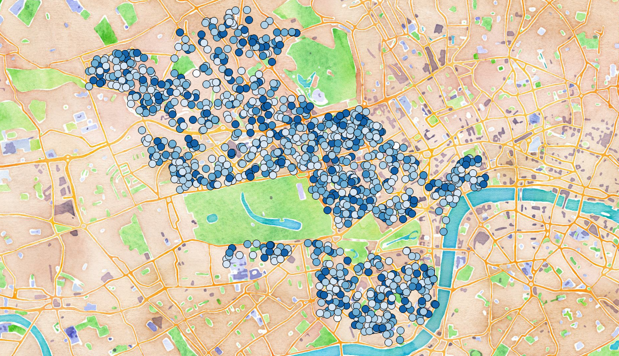
# plot free space for each location using a the size of a circle to indicate the number of free spaces
for tup in free_space_0.keys():
plt.plot(tup[1], tup[0], 'bo', ms = np.max([0,free_space_0[tup]/2]),alpha = (1 + float(tariff[tup]))/5.4)
plt.title('Westminster \n Unoccupied Parking Spaces')
plt.text(- 0.13, 51.53,'Mon ' + str(h).zfill(2) + ':' + str(m).zfill(2))
plt.xlabel('Longitude')
plt.ylabel('Latitude')
plt.show()

In [ ]:
# Finally, we can loop through different times to create a series of images for creating an animation


# set the time step for visualising occupancy
ts = 5
cnt = 0
for h in np.arange(0,24):
	for m in np.arange(0,60,ts):

        # Use the Tariff to set an alpha value so we can see which parking locations are more expensive
        tariff = p.minor_xs( u'Tariff').ix[datetime.time(h,m)]

        # get the free spaces for 12:30
        free_space_0 = mon_free_spaces.ix[datetime.time(h,m)]

        # plot free space for each location using a the size of a circle to indicate the number of free spaces
        for tup in free_space_0.keys():
            plt.plot(tup[1], tup[0], 'bo', ms = np.max([0,free_space_0[tup]/2]),alpha = (1 + float(tariff[tup]))/5.4)

        plt.title('Westminster \n Unoccupied Parking Spaces')
        plt.text(- 0.13, 51.53,'Mon ' + str(h).zfill(2) + ':' + str(m).zfill(2))
        plt.xlabel('Longitude')
        plt.ylabel('Latitude')

		cnt = cnt + 1
		fname = 'image' + str(cnt).zfill(5) + '.png'

		#print fname

		plt.savefig(fname)
		plt.clf()
In [26]:
from IPython.display import YouTubeVideo
YouTubeVideo('tW8o14Th8hw')
Out[26]:
In [23]:
# QGIS (visualisation of shapefiles backed by OpenLayers maps from Google and OSM)
from IPython.display import Image

Image(url = 'http://ianozsvald.com/wp-content/uploads/2013/10/whitehall_1to36_capacity_1341parkingbays_bytarrif.png')
Out[23]:
In [ ]: